An almost binomial Markov chain

Everybody knows how to toss a coin. This time we’ll toss it a few times.

A Bernoulli random variable

Recall that \(Y\sim \mathrm{Bernoulli}(p)\) if \(Y\) can attain values from the set \(\{0, 1\}\) with probability \(P(Y=1) = p\) and \(P(Y=0) = 1-p\). It’s easy to see that:

• For every \(k\ge 1\) the random variables \(Y^k\) and \(Y\) are equal.
• The expected value is \(\mathbb E[Y] = p\).
• The variance is \(\mathbb{V}[Y]=\mathbb E[Y^2]-\mathbb E[Y]^2 = p-p^2 = p(1-p).\) From AM-GM we see that \(\mathbb{V}[Y] \le (1/2)^2=1/4\).

Now, if we consider independent and identically distributed variables \(Y_1\sim \mathrm{Bernoulli}(p)\), \(Y_2\sim \mathrm{Bernoulli}(p)\), …, \(Y_n\sim \mathrm{Bernoulli}(p)\), we can define a new variable \(N_n = Y_1 + \cdots + Y_n\) and an average \[ \bar Y^{(n)} = \frac{N_n}{n}.\]

The random variable \(N_n\) is distributed according to the binomial distribution and it’s easy to calculate the mean \(\mathbb E[N_n] = np\) and variance \(\mathbb V[N_n] = np(1-p)\). Consequently, \(\mathbb E[ \bar Y^{(n)} ] = p\) and \(\mathbb V[\bar Y^{(n)}] = np(1-p)/n^2 = p(1-p)/n \le 1/4n\).

Hence, we see that if we want to estimate \(p\), then \(\bar Y^{(n)}\) is a reasonable estimator to use, and we can control its variance by choosing appropriate \(n\).

Thinking about very large \(n\), recall that the strong law of large numbers guarantees that \[ P\left( \lim\limits_{n\to \infty} \bar Y^{(n)} = p \right) = 1. \]

A bit lazy coin tossing

Above we defined a sequence of independent Bernoulli variables. Let’s introduce some dependency between them: define \[ Y_1\sim \mathrm{Bernoulli}(p) \] and, for \(n\ge 1\), \[ Y_{n+1}\mid Y_n \sim w\,\delta_{Y_n} +(1-w)\, \mathrm{Bernoulli}(p). \]

Hence, to draw \(Y_1\) we simply toss a coin, but to draw \(Y_2\) we can be lazy with probability \(w\) and use the sampled value \(Y_1\) or, with probability \(1-w\), actually do the hard work of tossing a coin again.

Let’s think about the marginal distributions, i.e., we observe only the \(n\)th coin toss. As \(Y_n\) takes values in \(\{0, 1\}\), it has to be distributed according to some Bernoulli distribution.

Of course, we have \(\mathbb E[Y_1] = p\), but what is \(\mathbb E[Y_2]\)? Using the law of total expectation we have \[ \mathbb E[Y_2] = \mathbb E[ \mathbb E[Y_2\mid Y_1] ] = \mathbb E[ w Y_1 + (1-w)p ] = p. \] Interesting! Even if we have large \(w\), e.g., \(w=0.9\), we will still see \(Y_2=1\) with original probability \(p\). More generally, we can prove by induction that that \(\mathbb E[Y_n] = p\) for all \(n\ge 1\).

To calculate the variance, we could try the law of total variance, but there is a simpler way: from the above observations we see that all the variables are distributed as \(Y_n\sim \mathrm{Bernoulli}(p)\) (so they are identically distributed, but not independent for \(w>0\)) and the variance has to be \(\mathbb V[Y_n] = p(1-p)\).

Let’s now introduce variables \(N_n = Y_1 + \cdots + Y_n\) and \(\bar Y^{(n)}=N_n/n\). As expectation is a linear operator, we know that \(\mathbb E[N_n] = np\) and \(\mathbb E[\bar Y^{(n)}]=p\), but how exactly are these variables distributed? Or, at least, can we say anything about their variance?

It’s instructive to see what happens for \(w=1\): intuitively, we only tossed the coin once, and then just “copied” the result \(n\) times, so that the sample size used to estimate \(\bar Y^{(n)}\) is still one.

More formally, with probability 1 we have \(Y_1 = Y_2 = \cdots = Y_n\), so that \(N_n = nY_1\) and \(\mathbb V[N_n] = n^2p(1-p)\). Then, also with probability 1, we also have \(\bar Y^{(n)}=Y_1\) and \(\mathbb V[\bar Y^{(n)}]=p(1-p)\).

More generally, we have \[ \mathbb V[N_n] = \sum_{i=1}^n \mathbb V[Y_i] + \sum_{i\neq j} \mathrm{cov}[Y_i, Y_j] \] and we can suspect that the covariance terms will be non-negative, usually incurring larger variance than a corresponding binomial distribution (obtained from independent draws). Let’s prove that.

Markov chain

We will be interested in covariance terms \[\begin{align*} \mathrm{cov}(Y_i, Y_{i+k}) &= \mathbb E[Y_i\cdot Y_{i+k}] - \mathbb E[Y_i]\cdot \mathbb E[Y_{i+k}] \\ &= P(Y_i=1, Y_{i+k}=1)-p^2 \\ &= P(Y_i=1)P( Y_{i+k}=1\mid Y_i=1) -p^2 \\ &= p\cdot P(Y_{i+k}=1 \mid Y_i=1) - p^2. \end{align*} \]

To calculate the probability \(P(Y_{i+k}=1\mid Y_i=1)\) we need an observation: the sampling procedure defines a Markov chain with the transition matrix \[ T = \begin{pmatrix} P(0\to 0) & P(0 \to 1)\\ P(1\to 0) & P(1\to 1) \end{pmatrix} = \begin{pmatrix} w+(1-w)(1-p) & p(1-w)\\ (1-w)(1-p) & w + p(1-w) \end{pmatrix}. \]

By induction and a handy identity \((1-x)(1+x+\cdots + x^{k-1}) = 1-x^{k}\) one can prove that \[ T^k = \begin{pmatrix} 1-p(1-w^k) & p(1-w^k)\\ (1-p)(1-w^k) & p+w^k(1-p), \end{pmatrix} \] from which we can conveniently read \[ P(Y_{i+k}=1\mid Y_i=1) = p+w^k(1-p) \] and \[\mathrm{cov}(Y_i, Y_{i+k}) = w^k\cdot p(1-p).\]

Great, these terms are always non-negative! Let’s do a quick check: for \(w=0\) the covariance terms vanish, resulting in \(\mathbb V[N_n]=np(1-p) + 0\) and for \(w=1\) we have \(\mathbb V[N_n] = np(1-p) + n(n-1)p(1-p)=n^2p(1-p)\).

For \(w\neq 1\) we can use the same identity as before to get \[\begin{align*} \mathbb V[N_n] &= p(1-p)\cdot \left(n+\sum_{i=1}^n \sum_{k=1}^{n-i} w^k \right) \\ &= p(1-p)\left( n+ \frac{2 w \left(w^n-n w+n-1\right)}{(w-1)^2} \right) \end{align*} \]

Let’s numerically check whether this formula seems right:

Code

from functools import partial

import jax
import jax.numpy as jnp
from jax import random, lax

@partial(jax.jit, static_argnames=["n"])
def simulate_markov_chain(key, n: int, p: float, w: float) -> jnp.ndarray:
    keys = random.split(key, n)

    def step(i, y):
        key_w, key_p = random.split(keys[i])
        y_prev = y[i-1]
        mixture_sample = random.bernoulli(key_w, w)
        y_next = jnp.where(mixture_sample, y_prev, random.bernoulli(key_p, p))
        y = y.at[i].set(y_next)
        return y
    
    y_init = jnp.zeros(n, dtype=jnp.int32)
    y_init = y_init.at[0].set(random.bernoulli(keys[0], p))

    y_final = lax.fori_loop(1, n, step, y_init)
    return y_final

def simulate_correlated_binomial(key, n: int, p: float, w: float) -> int: 
    return simulate_markov_chain(key=key, n=n, p=p, w=w).sum()

@partial(jax.jit, static_argnames=["n", "n_samples"])
def sample_correlated_binomial(key, n: int, p: float, w: float, n_samples: int = 1_000_000) -> jnp.ndarray:
    keys = random.split(key, n_samples)
    return jax.vmap(partial(simulate_correlated_binomial, n=n, p=p, w=w))(keys)

def variance_correlated_binomial(n: int, p: float, w: float) -> float:
    factor = n**2
    if w < 1.0:
        factor = n + ( 2 * w * (-1 + n - n * w + w**n)) / (-1 + w)**2
    return p*(1-p) * factor

key = random.PRNGKey(2024-1-19)

test_cases = [
    (10, 0.5, 0.5),
    (10, 0.3, 0.8),
    (10, 0.2, 0.1),
    (5, 0.4, 0.3),
    (20, 0.8, 0.7),
]

for n, p, w in test_cases:
    key, subkey = random.split(key)
    approx = jnp.var(sample_correlated_binomial(subkey, n, p, w))
    exact = variance_correlated_binomial(n, p, w)

    print(f"Variance (appr.): {approx:.2f}")
    print(f"Variance (exact): {exact:.2f}")
    print("-"*23)

An NVIDIA GPU may be present on this machine, but a CUDA-enabled jaxlib is not installed. Falling back to cpu.

Variance (appr.): 6.50
Variance (exact): 6.50
-----------------------
Variance (appr.): 11.40
Variance (exact): 11.40
-----------------------
Variance (appr.): 1.92
Variance (exact): 1.92
-----------------------
Variance (appr.): 1.93
Variance (exact): 1.94
-----------------------
Variance (appr.): 15.66
Variance (exact): 15.65
-----------------------

Markov chain Monte Carlo

Recall that when the samples are independent, we can estimate \(p\) via \(\bar Y^{(n)}\) which is an unbiased estimator, i.e., \(\mathbb E[\bar Y^{(n)}] = p\) and its variance is \(\mathbb V[\bar Y^{(n)}]=p(1-p)/n\le 1/4n\).

When we passed to a Markov chain introducing parameter \(w\), we also found out that \(\mathbb E[\bar Y^{(n)}]=p\). Moreover, for \(w<1\) (i.e., there’s some genuine sampling, rather than copying the first result) the variance of \(N_n\) also grows as \(\mathcal O(n + w^n)=\mathcal O(n)\), so that \(\mathbb V[\bar Y^{(n)}] =\mathcal O(1/n)\), so that for a large \(n\) the estimator \(\bar Y^{(n)}\) can be a reliable estimator for \(p\). However, note that in the variance there’s a term \(1/(1-w)^2\), so that for \(w\) close to \(1\) one may have to use very, very, very large \(n\) to make sure that the variance is small enough.

This Markov chain is in fact connected to Markov chain Monte Carlo samplers, used to sample from a given distribution.

The Markov chain \(Y_2, Y_3, \dotsc\) has transition matrix \(T\) and initial distribution of \(Y_1\) (namely \(\mathrm{Bernoulli}(p)\)). For \(0 < p < 1\) and \(w < 1\) the transition matrix has positive entries, which implies that this Markov chain is ergodic (both irreducibility and aperiodicity are trivially satisfied in this case; more generally quasi-positivity, i.e., \(T^k\) has positive entries for some \(k\ge 1\), is equivalent to ergodicity).

We can deduce two things. First, there’s a unique stationary distribution of this Markov chain. It can be found by solving the equations for the eigenvector \(T^{t}\pi=\pi\); in this case \(\pi=(1-p, p)\) (what a surprise!), meaning that the stationary distribution is \(\mathrm{Bernoulli}(p)\).

Secondly, we can use the ergodic theorem. The ergodic theorem states that in this case for every function¹ \(f\colon \{0, 1\}\to \mathbb R\) it holds that \[ P\left(\lim\limits_{n\to\infty} \frac{1}{n}\sum_{i=1}^n f(Y_i) = \mathbb E[f] \right) = 1 \] where the expectation \(\mathbb E[f]\) is taken with respect to \(\pi\).

Note that for \(f(x) = x\) we find out that with probability \(1\) it holds that \(\lim\limits_{n\to \infty} \bar Y^{(n)} = p\).

Perhaps it’s worth commenting on why the stationary distribution is \(\mathrm{Bernoulli}(p)\). Consider any distribution \(\mathcal D\) and a Markov chain \[ Y_{n+1} \mid Y_n \sim w\, \delta_{Y_{n}} + (1-w)\, \mathcal D \] for \(w < 1\). Intuitively, this Markov chain will either jump to a new location with the right probability, or stay at a current point by some additional time. This additional time depends only on \(w\), so that on average, at each point we spend the same time. Hence, it should not affect time averages over very, very, very long sequences. (However, as we have seen, large \(w\) may imply large autocorrelation in the Markov chain and the chain would have to be extremely long to yield acceptable variance).

I think it should not be hard to formalize and prove the above observation, but it’s not for today. This review could be useful for investigating this further.

How does it differ from beta-binomial?

Recall that a beta-binomial distribution generates samples as follows:

1. Draw \(b\sim \mathrm{Beta}(\alpha, \beta)\);
2. Then, draw \(M \mid b \sim \mathrm{Binomial}(n, b)\).

Hence, first a random coin is selected from a set of coins with different biases, and then it’s tossed \(n\) times. This distribution has two degrees of freedom: \(\alpha\) and \(\beta\), and allows one a more flexible control over both the mean and the variance. The mean is given by \[ \mathbb E[M] = n\frac{\alpha}{\alpha + \beta}, \] so if we write \(p = \alpha/(\alpha + \beta)\), we match the mean of a “corresponding” binomial distribution. The variance is given by \[ \mathbb V[M] = np(1-p)\left(1 + \frac{n-1}{\alpha + \beta + 1} \right), \] so that for \(n \ge 2\) we will see a larger variance than for a binomial distribution with corresponding mean.

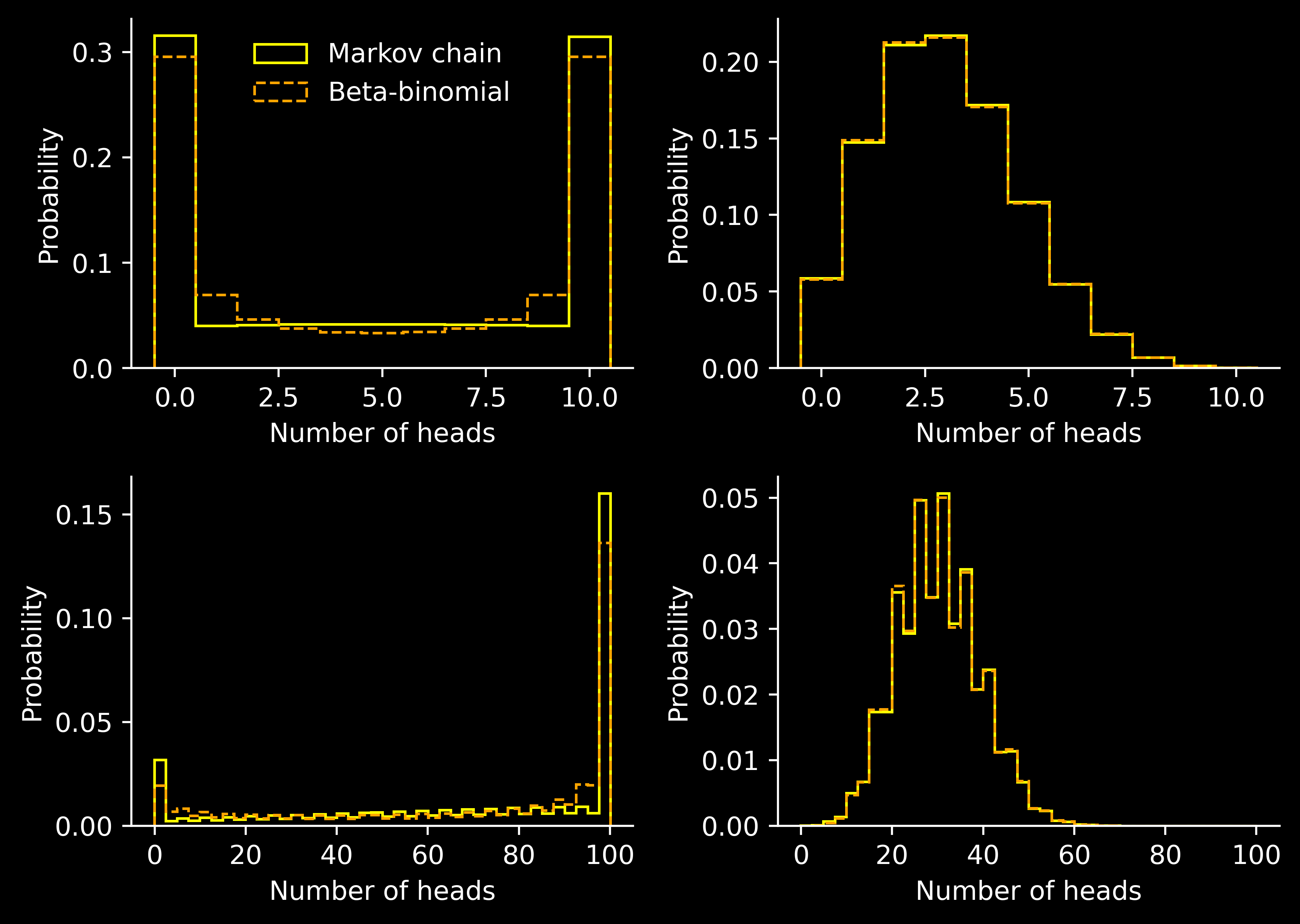
We see that this variance is quadratic in \(n\), which is different from the formula for the variance of the almost binomial Markov chain. Nevertheless, we can ask ourselves a question whether beta-binomial can be a good approximation to the distribution studied before.

This intuition may be formalized in many ways, e.g., as minimization of statistical discrepancy measures, including total variation, various Wasserstain distances or \(f\)-divergences. Instead, we will just match mean and variance.

So, of course, we will take \(p=\alpha/(\alpha + \beta)\) and additionally solve for \(\mathbb V[M] = V\). The solution is then given by \[\begin{align*} \alpha &= pR,\\ \beta &= (1-p)R,\\ R &= \frac{n^2 p(1-p)-V}{V - n p(1-p)}. \end{align*} \]

Now it’s coding time! We could use TensorFlow Probability on JAX to sample from beta-binomial distribution, but we will resort to core JAX.

Code

import matplotlib.pyplot as plt 
plt.style.use("dark_background")

def find_alpha_beta(n: int, p: float, variance: float) -> tuple[float, float]:
    num = n**2 * p * (1-p) - variance
    den = variance - n * p * (1-p)
    r = num / den

    if r <= 0 or p <= 0 or p >= 1:
        raise ValueError("Input results in non-positive alpha or beta")

    return p*r, (1-p) * r

@partial(jax.jit, static_argnames=["n"])
def _sample_beta_binomial(key, n: int, alpha: float, beta: float) -> int:
    key_p, key_b = random.split(key)
    p = random.beta(key_p, a=alpha, b=beta)
    ber = random.bernoulli(key_b, p=p, shape=(n,))
    return jnp.sum(ber)

@partial(jax.jit, static_argnames=["n", "n_samples"])
def sample_beta_binomial(key, n: int, alpha: float, beta: float, n_samples: int = 1_000_000) -> jnp.ndarray:
    keys = random.split(key, n_samples)
    return jax.vmap(partial(_sample_beta_binomial, n=n, alpha=alpha, beta=beta))(keys)


def plot_compare(key, ax: plt.Axes, n: int, p: float, w: float, n_samples: int = 1_000_000, n_bins: int | None = None) -> None:
    variance = variance_correlated_binomial(n=n, p=p, w=w)
    alpha, beta = find_alpha_beta(n=n, p=p, variance=variance)

    key1, key2 = random.split(key)
    sample_corr = sample_correlated_binomial(key1, n=n, p=p, w=w, n_samples=n_samples)
    sample_betabin = sample_beta_binomial(key2, n=n, alpha=alpha, beta=beta, n_samples=n_samples)

    if n_bins is None:
        bins = jnp.arange(-0.5, n + 1.5, 1)
    else:
        bins = jnp.linspace(-0.1, n + 0.1, n_bins)

    ax.hist(
        sample_corr, bins=bins, density=True, rasterized=True,
        color="yellow",
        label="Markov chain",
        histtype="step",
    )
    ax.hist(
        sample_betabin, bins=bins, density=True, rasterized=True,
        color="orange",
        label="Beta-binomial",
        histtype="step",
        linestyle="--"
    )
    ax.spines[["top", "right"]].set_visible(False)
    ax.set_xlabel("Number of heads")
    ax.set_ylabel("Probability")


fig, _axs = plt.subplots(2, 2, dpi=250)
axs = _axs.ravel()

key, *keys = random.split(key, 1 + len(axs))

params = [
    # (n, p, w, n_bins)
    (10, 0.5, 0.9, None),
    (10, 0.3, 0.2, None),
    (100, 0.7, 0.98, 41),
    (100, 0.3, 0.6, 41),
]
assert len(params) == len(axs)

for key, ax, (n, p, w, n_bins) in zip(keys, axs, params):
    plot_compare(
        key=key,
        ax=ax,
        n=n,
        p=p,
        w=w,
        n_samples=1_000_000,
        n_bins=n_bins,
)
axs[0].legend(frameon=False)
fig.tight_layout()

Footnotes

1. Usually one has to add that the function is bounded. But we are working with a finite domain \(\{0, 1\}\), so literally every function is bounded.