Starting (on finite domains) with Gaussian processes

Gaussian processes are wonderful. Let’s take a look at the machinery behind them in the simplest case: when they are just a multivariate normal distribution.

Let \(Y = (Y_1, \dotsc, Y_n)^T\) be a random variable distributed according to the multivariate normal distribution \(\mathcal N(\mu, \Sigma)\), where \(\mu\in \mathbb R^n\) and \(\Sigma\) is a real symmetric positive-definite¹ \(n\times n\) matrix.

We will think of this distribution in the following manner: we have a domain \(\mathcal X = \{1, 2, \dotsc, n\}\) and for each \(x\in \mathcal X\) we have a random variable \(Y_i\) and the joint distribution \(P(Y_1, \dotsc, Y_n)\) is multivariate normal.

Assume that we have measured \(Y_x\) variables for indices \(x_1, \dotsc, x_k\), with corresponding values \(Y_{x_1}=y_1, \dotsc, Y_{x_k}=y_k\), and we are interested in predicting the values at locations \(x'_1, \dotsc, x'_q\), i.e., modelling the conditional probability distribution \[ P(Y_{x'_1}, \dotsc, Y_{x'_q} \mid Y_{x_1}=y_1, \dotsc, Y_{x_k}=y_k). \]

We will also allow \(k=0\), i.e., we would like to access marginal distributions. This can be treated as an extension of the problems answered by bend and mix models we studied here.

Formalising the problem

To formalise the problem a bit:

Conditional calculation

Consider a set of measured values \(M = \{(x_1, y_1), \dotsc, (x_k, y_k)\}\) and a non-empty query set \(Q = \{x'_1, \dotsc, x'_q\} \subseteq \mathcal X\).

We assume that \(Q\cap M_x = \varnothing\) and \(|M_x| = |M|\), where \(M_x = \{x \in \mathcal X \mid (x, y)\in M \text{ for some } y \}\).

We would like to be able to sample from the conditional probability distribution \[ P(Y_{x_1'}, \dotsc, Y_{x_q'} \mid Y_{x_1}=y_1, \dotsc, Y_{x_k}=y_k) \] as well as to evaluate the (log-)density at any point.

We allow \(M=\varnothing\), which corresponds then to marginal distributions.

This problem can be solved for multivariate normal distributions by noticing that all conditional (and marginal) distributions will also be multivariate normal. Let’s introduce some notation.

For a tuple \(\pi = (\pi_1, \dotsc, \pi_m) \in \mathcal X^m\) such that \(\pi_i\neq \pi_j\) for \(i\neq j\), we will write \(Y_\pi\) for a random vector \((Y_{\pi_1}, \dotsc, Y_{\pi_m})\). Note that this operation can be implemented using a linear mapping \(A_\pi \colon \mathbb R^n\to \mathbb R^m\) with \[ A_\pi \begin{pmatrix} Y_1 \\ \vdots \\ Y_n \end{pmatrix} = \begin{pmatrix} Y_{\pi_1} \\ \vdots \\ Y_{\pi_m} \end{pmatrix} \] and \((A_\pi)_{oi} = \mathbf 1[ i = \pi_o]\). Hence, \(Y_\pi\) vector is distributed according to \(\mathcal N(A_\pi\mu, A_\pi\Sigma A_\pi^T)\).

The above operation suffices for calculating arbitrary marginal distributions and distributions corresponding to permuting the components.

Consider now the case where we want to calculate a “true” conditional distribution (i.e., with \(M\neq \varnothing\)), so the marginalisation does no suffice.

We can use the tuple \(\pi = (x_1', \dotsc, x_q', x_1, \dotsc, x_k)\) to select the right variables and reorder them into a \(q\)-dimensional block of unobserved (“query”) variables and a \(k\)-dimensional block of observed (“key”) variables².

Conditioning multivariate normal

Let \(Y=(Y_1, Y_2) \in \mathbb R^{k}\times \mathbb R^{n-k}\) be a random vector split into blocks of dimensions \(k\) and \(n-k\). If \(Y\sim \mathcal N(\mu, \Sigma)\), where \[ \mu = (\mu_1, \mu_2) \] and \[ \Sigma = \begin{pmatrix} \Sigma_{11} & \Sigma_{12} \\ \Sigma_{21} & \Sigma_{22} \end{pmatrix}, \]

then for every \(y \in \mathbb R^{n-k}\) it holds that

\[ Y_1 \mid Y_2=y \sim \mathcal N(\mu', \Sigma'), \] where \[ \mu' = \mu_1 + {\color{Apricot}\Sigma_{12}\Sigma_{22}^{-1}}(y-\mu_2) \] and \[ \Sigma' = \Sigma_{11} - {\color{Apricot}\Sigma_{12} \Sigma_{22}^{-1}} \Sigma_{21}. \]

We see that in both formulae the matrix of regression coefficients³ \(\color{Apricot}\Sigma_{12}\Sigma_{22}^{-1}\) appears. We will discuss calculation of this term below.

Let’s write some code

Now let’s implement a prototype:

Code

import numpy as np
import numpy.linalg as npla
from jaxtyping import Float, Int, Array

from scipy import stats
import scipy.linalg as spla


class MultivariateNormal:
  def __init__(
    self,
    mu: Float[Array, " dim"],
    cov: Float[Array, "dim dim"],
  ) -> None:
    eigvals, _ = npla.eig(cov)
    if np.min(eigvals) <= 0:
      raise ValueError(f"Covariance should be positive-definite.")
    
    self.mu = np.asarray(mu)
    self.cov = np.asarray(cov)
    dim = self.mu.shape[0]

    assert self.mu.shape == (dim,)
    assert self.cov.shape == (dim, dim)

  @property
  def dim(self) -> int:
    return self.mu.shape[0]

  def sample(
    self,
    rng: np.random.Generator,
    size: int = 1,
  ) -> np.ndarray:
    return rng.multivariate_normal(
      mean=self.mu, cov=self.cov, size=size,
    )

  def logpdf(self, y: Float[Array, " dim"]) -> float:
    return stats.multivariate_normal.logpdf(
      y,
      mean=self.mu,
      cov=self.cov,
      allow_singular=False,
    )


def _contruct_projection_matrix(
  n: int,
  indices: Int[Array, " k"],
) -> Int[Array, "k n"]:
  indices = np.asarray(indices, dtype=int)  

  # Output dimension
  k = indices.shape[0]
  if np.unique(indices).shape[0] != k:
    raise ValueError("Indices should be unique.")

  inp = np.arange(n, dtype=int)
  
  ret = np.asarray(inp[None, :] == indices[:, None], dtype=int)
  assert ret.shape == (k, n)
  return ret


def select(
  dist: MultivariateNormal,
  indices: Int[Array, " k"],
) -> MultivariateNormal:
  proj = np.asarray(
    _contruct_projection_matrix(
      n=dist.dim,
      indices=indices,
    ),
    dtype=float,
  )
  
  new_mu = np.einsum("oi,i -> o", proj, dist.mu)
  new_cov = np.einsum("oi,iI,OI -> oO", proj, dist.cov, proj)
  
  return MultivariateNormal(
    mu=new_mu,
    cov=new_cov,
  )

def _regression_coefs(
  sigma12: Float[Array, "Q K"],
  sigma22: Float[Array, "K K"],
) -> Float[Array, "Q K"]:
  return spla.solve(sigma22, sigma12.T).T

def _condition_gaussian(
  dist: MultivariateNormal,
  m: int,
  y: Float[Array, " vals"]
) -> MultivariateNormal:
  assert y.shape[0] == dist.dim - m

  mu1 = dist.mu[:m]
  mu2 = dist.mu[m:]
  sigma11 = dist.cov[:m, :m]
  sigma12 = dist.cov[:m, m:]
  sigma22 = dist.cov[m:, m:]

  reg = _regression_coefs(
    sigma12=sigma12, sigma22=sigma22,
  )

  mu_ = mu1 + reg @ (y - mu2)
  sigma_ = sigma11 - reg @ sigma12.T

  return MultivariateNormal(
    mu=mu_, cov=sigma_,
  )

def condition(
  dist: MultivariateNormal,
  query: Int[Array, " Q"],
  key: Int[Array, " K"],
  values: Float[Array, " K"],
) -> MultivariateNormal:
  q, k = query.shape[0], key.shape[0]
  assert values.shape == (k,), "Values have wrong shape"

  total_index = np.concatenate((query, key))

  if np.unique(total_index).shape[0] != k + q:
    raise ValueError("Indices must be unique.")
  if np.min(total_index) < 0 or np.max(total_index) >= dist.dim:
    raise ValueError("Indices must be from the set 0, 1, ..., dim-1.")

  ordered_dist = select(dist, indices=total_index)

  if k == 0:
    return ordered_dist
  else:
    return _condition_gaussian(
      dist=ordered_dist,
      m=q,
      y=values,
    )

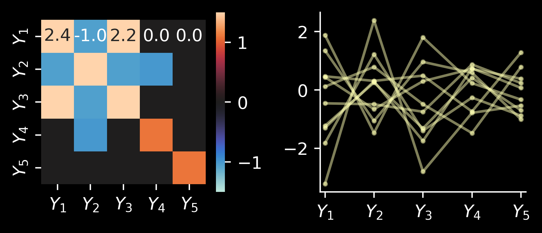
Now we can do conditioning. For example, imagine that we have \(\mu = 0\) and we know \(\Sigma\): \(Y_1\) correlates with \(Y_3\), and \(Y_2\) anticorrelates with \(Y_4\) and \(Y_5\) doesn’t correlate with anything else. We measure \(Y_1\) and \(Y_2\), so we can use this correlation structure to impute \(Y_3\), \(Y_4\) and \(Y_5\).

First, let’s plot the covariance matrix and the samples:

Code

import matplotlib.pyplot as plt
import seaborn as sns
plt.style.use("dark_background")

mixing = np.asarray([
  [1.5, -0.7, 1.5, 0, 0],
  [0, 1, 0, -1, 0],
  [0, 0, 0, 0, 1],
], dtype=float)

cov = np.einsum("io,iO->oO", mixing, mixing) + 0.1 * np.eye(5)

fig, axs = plt.subplots(1, 2, figsize=(4.5, 2), dpi=200)
ticklabels = [f"$Y_{i}$" for i in range(1, 5+1)]

ax = axs[0]
sns.heatmap(cov, ax=ax, xticklabels=ticklabels, yticklabels=ticklabels, vmin=-1.5, vmax=1.5, center=0, square=True, annot=True, fmt=".1f")

dist = MultivariateNormal(mu=np.zeros(5), cov=cov)
rng = np.random.default_rng(42)
samples = dist.sample(rng, size=10)

ax = axs[1]
for sample in samples:
  x_ax = np.arange(1, 6)
  ax.plot(x_ax, sample, alpha=0.5, c="C1")
  ax.scatter(x_ax, sample, alpha=0.5, c="C1", s=4)

ax.spines[['top', 'right']].set_visible(False)
ax.set_xlim(0.9, 5.1)
ax.set_xticks(x_ax, ticklabels)

fig.tight_layout()

Imagine now that we observed \(Y_1=1.5\) and \(Y_2=1\). We expect that \(Y_3\) should move upwards (the posterior should be shifted so that most of the mass is above \(0\)), \(Y_4\) to go downwards and \(Y_5\) to stay as it was. Let’s plot covariance matrix and draws from the conditional posterior \(P(Y_3, Y_4, Y_5\mid Y_1=1.5, Y_2=1)\):

Code

y_obs = np.asarray([1.5, 1])
cond = condition(
  dist=dist,
  query=np.asarray([2, 3, 4]),
  key=np.asarray([0, 1]),
  values=y_obs,
)

fig, axs = plt.subplots(1, 2, figsize=(4.5, 2), dpi=200)

ax = axs[0]
sns.heatmap(
  cond.cov,
  ax=ax,
  xticklabels=ticklabels[2:],
  yticklabels=ticklabels[2:],
  vmin=-1.5,
  vmax=1.5,
  center=0,
  annot=True,
  square=True,
)

ax = axs[1]
ax.spines[['top', 'right']].set_visible(False)
ax.set_xlim(0.9, 5.1)
ax.set_xticks(x_ax)

ax.scatter([1, 2], y_obs, c="maroon", s=4)

samples = cond.sample(rng, size=10)
for sample in samples:
  ax.plot([3, 4, 5], sample, alpha=0.5, c="C1")
  ax.scatter([3, 4, 5], sample, alpha=0.5, c="C1", s=4)

ax.set_xticks(x_ax, ticklabels)

fig.tight_layout()

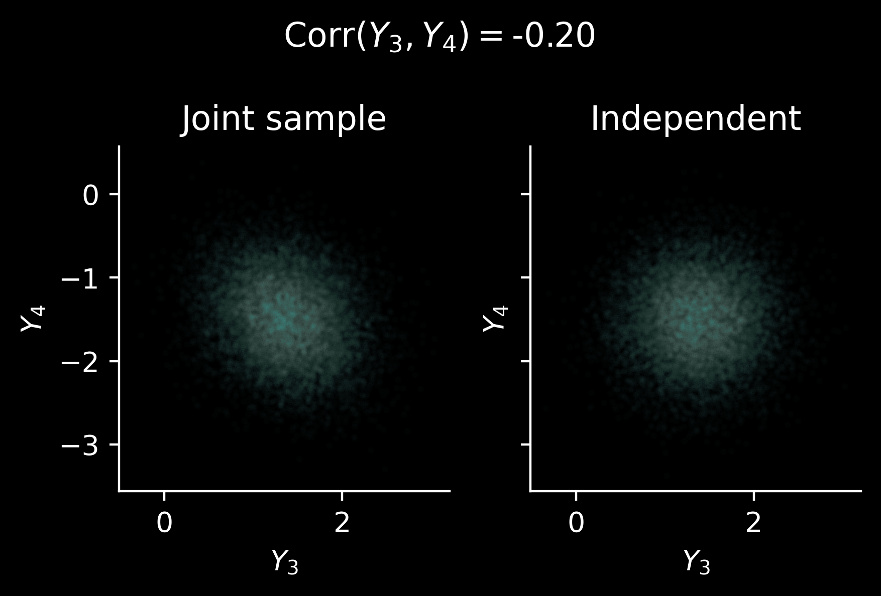
We see that there is slight anticorrelation between \(Y_3\) and \(Y_4\): by sampling from the conditional distribution we obtain a coherent sample. This is different than drawing independent samples from \(P(Y_3 \mid Y_1=y_1, Y_2=y_2)\) and \(P(Y_4\mid Y_1=y_1, Y_2=y_2)\). Perhaps it’ll be easier to visualise it on a scatter plot:

Code

fig, axs = plt.subplots(1, 2, figsize=(4.5, 3), dpi=200, sharex=True, sharey=True)
samples = cond.sample(rng, size=15_000)

ax = axs[0]
ax.scatter(samples[:, 0], samples[:, 1], s=2, alpha=0.01)
ax.set_title("Joint sample")
ax.set_xlabel(r"$Y_3$")
ax.set_ylabel(r"$Y_4$")

ax = axs[1]
samples2 = cond.sample(rng, size=samples.shape[0])
ax.scatter(samples[:, 0], samples2[:, 1], s=2, alpha=0.01)
ax.set_title("Independent")
ax.set_xlabel(r"$Y_3$")
ax.set_ylabel(r"$Y_4$")

corr = cond.cov[0, 1] / np.sqrt(cond.cov[0, 0] * cond.cov[1, 1])
fig.suptitle(r"$\text{Corr}(Y_3, Y_4) = $" + f"{corr:.2f}")
fig.tight_layout()

for ax in axs:
  ax.spines[['top', 'right']].set_visible(False)

Ok, it’s hard to see, but visible – the (negative) correlation is just quite weak in this case.

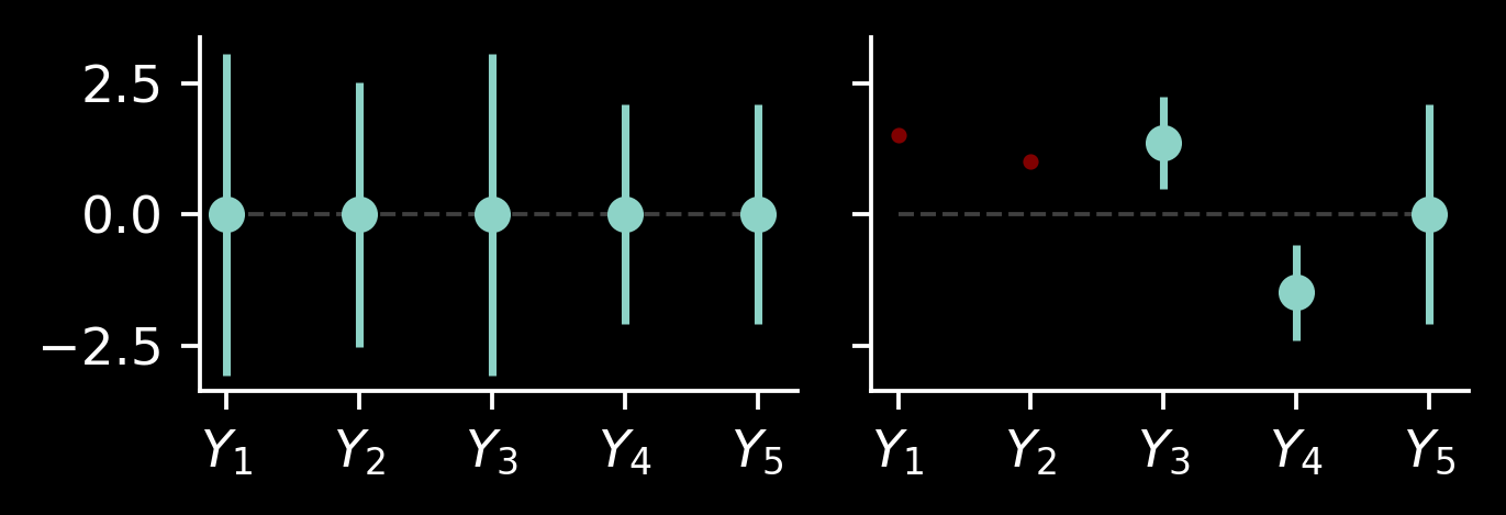
Let’s do the last visualisation before we move to Gaussian processes. As mentioned, the magical thing is the access to the whole posterior distribution \(P(Y_3, Y_4, Y_5 \mid Y_1=y_1, Y_2=y_2)\): we can evaluate arbitrary probabilities and sample consistent vectors from this distribution. We can visualise samples, but sometimes a simpler summary statistic would be useful. Each of the distributions \(P(Y_i \mid Y_1=y_1, Y_2=y_2)\) is one-dimensional Gaussian, so we can plot its mean and standard deviation. Or, even better, let’s plot \(\mu_i\pm 2\sigma_i\) to see where approximately 95% of probability lies.

We’ll plot these regions both before and after conditioning:

Code

fig, axs = plt.subplots(1, 2, figsize=(4, 1.5), dpi=170, sharex=True, sharey=True)

# Before conditioning
ax = axs[0]

ax.plot(np.arange(1, 1+5), np.zeros(5), linestyle="--", c="gray", alpha=0.5, linewidth=0.8)

ax.errorbar(
  np.arange(1, 1+5),
  dist.mu,
  yerr=2 * np.sqrt(np.diagonal(dist.cov)),
  fmt="o",
)

# After conditioning
ax = axs[1]
ax.plot(np.arange(1, 1+5), np.zeros(5), linestyle="--", c="gray", alpha=0.5, linewidth=0.8)
ax.scatter([1, 2], y_obs, c="maroon", s=4)
ax.errorbar(
  [3, 4, 5],
  cond.mu,
  yerr=2 * np.sqrt(np.diagonal(cond.cov)),
  fmt="o",
)

for ax in axs:
  ax.spines[['top', 'right']].set_visible(False)
  ax.set_xlim(0.8, 5.3)
  ax.set_xticks(x_ax, ticklabels)

fig.tight_layout()

As mentioned, these plots don’t really allow us to look at correlations between different variables, but they are still useful: we can easily see that the posterior of \(Y_3\) moved upwards and \(Y_4\) moved downwards! Variable \(Y_5\), which is independent of \((Y_1, Y_2, Y_3, Y_4)\), doesn’t change: if we want to know it, we just have to measure it.

Gaussian processes

For \(\mathcal X = \{1, \dotsc, n\}\) we considered an indexed collection of random variables \(\{Y_x\}_{x\in \mathcal X}\). Let’s call it a stochastic process.

This stochastic process has the property that the joint distribution over all variables was multivariate normal. From that we could deduce that distributions \(P(Y_{x_1}, \dotsc, Y_{x_m})\) were again multivariate normal, what in turn allowed us to do prediction via conditioning (which resulted, again, in multivariate normal distributions).

Let’s move beyond a finite dimension: take \(\mathcal X=\mathbb R\) and consider a stochastic process \(\{Y_x\}_{x\in \mathcal X}\). We will say that it’s a Gaussian process if for every finite set \(\{x_1, \dotsc, x_m\}\subseteq \mathcal X\) the joint distribution \(P(Y_{x_1}, \dotsc, Y_{x_m})\) is multivariate normal. More generally, we can take other domains \(\mathcal X\) (e.g., \(\mathbb R^n\)) and speak of Gaussian random fields.

In either case, the trick is that we never work with infinitely many random variables at once: for example, if we observe values \(y_1, \dotsc, y_k\) at locations \(x_1, \dotsc, x_k\) and we want to predict the values at points \(x'_1, \dotsc, x'_q\), we will construct the joint multivariate normal distribution \(P(Y_{x_1}, \dotsc, Y_{x_m}, Y_{x'_1}, \dotsc, Y_{x'_q})\) and condition on observed values to get the conditional distribution \(P(Y_{x'_1}, \dotsc, Y_{x'_q} \mid Y_{x_1} = y_1, \dotsc, Y_{x_k}=y_k)\).

Now the questions is: how can we define a consistent stochastic process with these great properties? When \(\mathcal X\) was finite, we could just define the joint probability distribution over all variables via mean and covariance. But now \(\mathcal X\) is not finite!

Consider therefore two functions, giving the mean and covariance: \(m \colon \mathcal X\to \mathbb R\) and \(k\colon \mathcal X\to \mathcal X\to \mathbb R^+\). The premise is to build multivariate normal distributions \(P(Y_{x_1}, \dotsc, Y_{x_m})\) by using the mean vector \(\mu_i = m(x_i)\) and covariance matrix \(\Sigma_{ij} = k(x_i, x_j)\).

First of all, we see that not all covariance functions are suitable: we want covariance matrices to be symmetric and positive-definite, so we should use positive-definite kernels.

Secondly, we don’t know if these probability distributions can be coherently glued to a stochastic process. The answer to this problem is provided by Daniell-Kolmogorov extension theorem, which says when a family of probability distributions can be coherently glued yielding a stochastic process. In this case parameterising covariances via \(\Sigma_{ij}=k(x_i, x_j)\) has the properties mentioned in the theorem. On the other hand, parameterising precision matrices via \(k(x_i, x_j)\) doesn’t generally yield a coherent stochastic process.

There are many important technical details, which I should mention here. Instead, I’ll refer to a great introduction to Gaussian processes at Dan Simpson’s blog, and implement something.

Modelling functions

There are many libraries for working with Gaussian processes, including GPJax, GPyTorch and GPy. We will however just use the code developed above, plus some simple covariance functions.

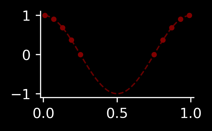
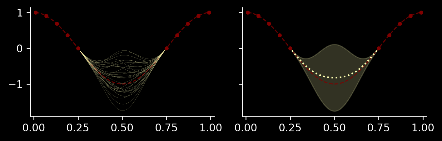
Our task will be the following: we are given some function on the interval \((0, 1)\). We observe some values \(M=\{(x_1, y_1), \dotsc, (x_k, y_k)\}\) inside the intervals \((0, u)\) and \((1-u, 1)\) and we want to predict the function behaviour in the interval \((u, 1-u)\), from which we do not have any data.

Code

import matplotlib.pyplot as plt
import dataclasses

@dataclasses.dataclass
class Task:
  xs_all: Float[Array, " points"]
  ys_all: Float[Array, " points"]
  xs_obs: Float[Array, " key"]
  ys_obs: Float[Array, " key"]
  xs_query: Float[Array, " query"]

def create_task(
  f,
  thresh: float = 0.25,
  k_2: int = 5,
  n_query: int = 101,
) -> Task:
  assert 0.02 < thresh < 0.98, "Threshold should be in (0.02, 0.98)"

  xs_all = np.linspace(0.01, 1)
  
  xs_obs = np.concatenate((np.linspace(0.01, thresh, k_2), np.linspace(1 - thresh, 0.99, k_2)))
  xs_query = np.linspace(thresh + 0.01, 0.99 - thresh, n_query)

  return Task(
    xs_all=xs_all,
    ys_all=f(xs_all),
    xs_obs=xs_obs,
    ys_obs=f(xs_obs),
    xs_query=xs_query,
  )

def plot_task(ax: plt.Axes, task: Task):
  ax.plot(
    task.xs_all, task.ys_all, linestyle="--", c="maroon", linewidth=1.0, alpha=0.8
  )
  ax.scatter(task.xs_obs, task.ys_obs, s=8, c="maroon")
  ax.spines[['top', 'right']].set_visible(False)
  ax.set_xlim(-0.02, 1.02)


fig, ax = plt.subplots(figsize=(2.2, 1.4), dpi=200)

task1 = create_task(lambda x: np.cos(2*np.pi * x))
plot_task(ax, task1)
fig.tight_layout()

We can approach this problem in two ways: first, we can impute missing values evaluated at some points.

For example, we can define a grid over \((u, 1-u)\) with \(q\) query points \(x'_1, \dotsc, x'_q\) and sample from the conditional distribution \(P(Y_{x'_1}, \dotsc, Y_{x'_q} \mid Y_{x_1}=y_1, \dotsc, Y_{x_k}=y_k)\) several times. This is one good way of plotting, showing us the behaviour of the whole sample at once.

Another way of plotting, which we also have already seen, is to take a single point \(x'\) and look at the normal distribution \(P(Y_{x'} \mid Y_{x_1}=y_1, \dotsc, Y_{x_k}=y_k)\), summarized by the mean and standard deviation: we can plot \(\mu(x') \pm 2\sigma(x')\) as a function of \(x'\) (similarly to the finite-dimensional case). This approach doesn’t allow us to look at joint behaviour at different locations, but is quite convenient to summarise uncertainty at a single specific point. For example, this may be informative enough to determine a good location of the next sample to collect in Bayesian optimisation framework (unless one wants to consider multiple points).

Let’s implement an example kernel and plot predictions in both ways:

Code

def kernel(x, x_):
  return np.exp(-20 * np.square(x-x_))

fig, axs = plt.subplots(1, 2, figsize=(2*3, 2), dpi=120, sharex=True, sharey=True)

for ax in axs:
  plot_task(ax, task1)

xs_eval = np.concatenate((task1.xs_query, task1.xs_obs))

cov = kernel(xs_eval[:, None], xs_eval[None, :]) + 1e-6 * np.eye(len(xs_eval))
dist = MultivariateNormal(np.zeros_like(xs_eval), cov)

cond = condition(
  dist=dist,
  query=np.arange(len(task1.xs_query)),
  key=np.arange(len(task1.xs_query), len(xs_eval)),
  values=task1.ys_obs
)

rng = np.random.default_rng(1)
samples = cond.sample(rng, size=30)

ax = axs[0]
for sample in samples:
  ax.plot(task1.xs_query, sample, alpha=0.8, color="C1", linewidth=0.1)


ax = axs[1]
ax.plot(task1.xs_query, cond.mu, c="C1", linestyle=":")
uncert = 2 * np.sqrt(np.diagonal(cond.cov))
ax.fill_between(task1.xs_query, cond.mu - uncert, cond.mu + uncert, color="C1", alpha=0.2)

fig.tight_layout()

Nice! I’ve been thinking about showing how different kernels result in differing predictions. But this post is already a bit too long, so I may write another one on this topic. In any case, there’s a Kernel Cookbook created by David Duvenaud.

Appendix

Matrix of regression coefficients

Let’s take a quick look at the matrix of regression coefficients, \(\Sigma_{12}\Sigma_{22}^{-1}\).

We could implement it via inversion, but there is a better solution.

Namely, note that if \(X=\Sigma_{12} \Sigma_{22}^{-1}\), then

\[ \Sigma_{22} X^T = \Sigma_{22} \Sigma_{22}^{-1} \Sigma_{12}^T = \Sigma_{12}^T \]

Hence, \(X^T\) is a solution to a matrix equation, which we can implement using scipy.linalg.solve. This is considered a better practice as it increases the numerical precision and can be faster (which is visible for large matrices; for small matrices the solution using matrix inversion was often faster).

Code

import time
import numpy as np
import numpy.linalg as npla
import scipy.linalg as spla


def calc_inv(sigma_12, sigma_22):
  return sigma_12 @ npla.inv(sigma_22)


def calc_solve(sigma_12, sigma_22):
  return spla.solve(sigma_22, sigma_12.T).T

rng = np.random.default_rng(42)

n_examples = 3
size = 20
m = 10

_coefs = rng.normal(size=(n_examples, size, size))
sigmas = np.einsum("kab,kac->kbc", _coefs, _coefs)
for sigma in sigmas:
  assert np.min(npla.eigvals(sigma)) > 0

  sigma_12 = sigma[:m, m:]
  sigma_22 = sigma[m:, m:]

  sol1 = calc_inv(sigma_12, sigma_22)
  sol2 = calc_solve(sigma_12, sigma_22)

  assert np.allclose(sol1, sol2), "Solutions differ."

Footnotes

1. For every non-zero \(x\in \mathbb R^n\) we have \(x^T\Sigma x > 0\), where the inequality is strict. As \(\Sigma\) is a real symmetric matrix, one of the versions of the spectral theorem yields a decomposition \(\Sigma = R^TDR\) for a diagonal matrix \(D\) and orthogonal \(R\). Hence, equivalently, we all eigenvalues have to be positive. See this link for more discussion.

2. I like to call them “query”, “keys” and “values” vectors, which makes the language a bit more similar to transformers. From that we just need one conditioning operation:

3. Why is it called in this manner? What are the slopes of \(\mu'\) change, when we vary observed values \(y\)?