Expectation-maximization and Gibbs sampling in quantification

Let’s analyse how to estimate how many cats and dogs can be found in an unlabeled data set.

Author

Paweł Czyż

Published

January 21, 2024

Consider an unlabeled image data set \(x_1, \dotsc, x_N\). We know that each image in this data set corresponds to a unique class (e.g., a cat or a dog) \(y\in \{1, \dotsc, L\}\) and we would like to estimate how many images \(x_i\) belong to each class. This problem is known as quantification and there exist numerous approaches to this problem, employing an auxiliary data set. Albert Ziegler and I were interested in additionally quantifying uncertainty¹ around such estimates (see Ziegler and Czyż 2023) by building a generative model on summary statistic and performing Bayesian inference.

We got a very good question from the reviewer: if we compare our method to point estimates produced by an expectation-maximization algorithm (Saerens, Latinne, and Decaestecker 2001) and we are interested in uncertainty quantification, why don’t we upgrade this method to a Gibbs sampler?

I like this question, because it’s very natural to ask, yet I overlooked the possibility of doing it. As Richard McElreath explains here, Hamiltonian Markov chain Monte Carlo is usually the preferred way of sampling, but let’s see how exactly the expectation-maximization algorithm works in this case and how to adapt it to a Gibbs sampler.

Modelling assumptions

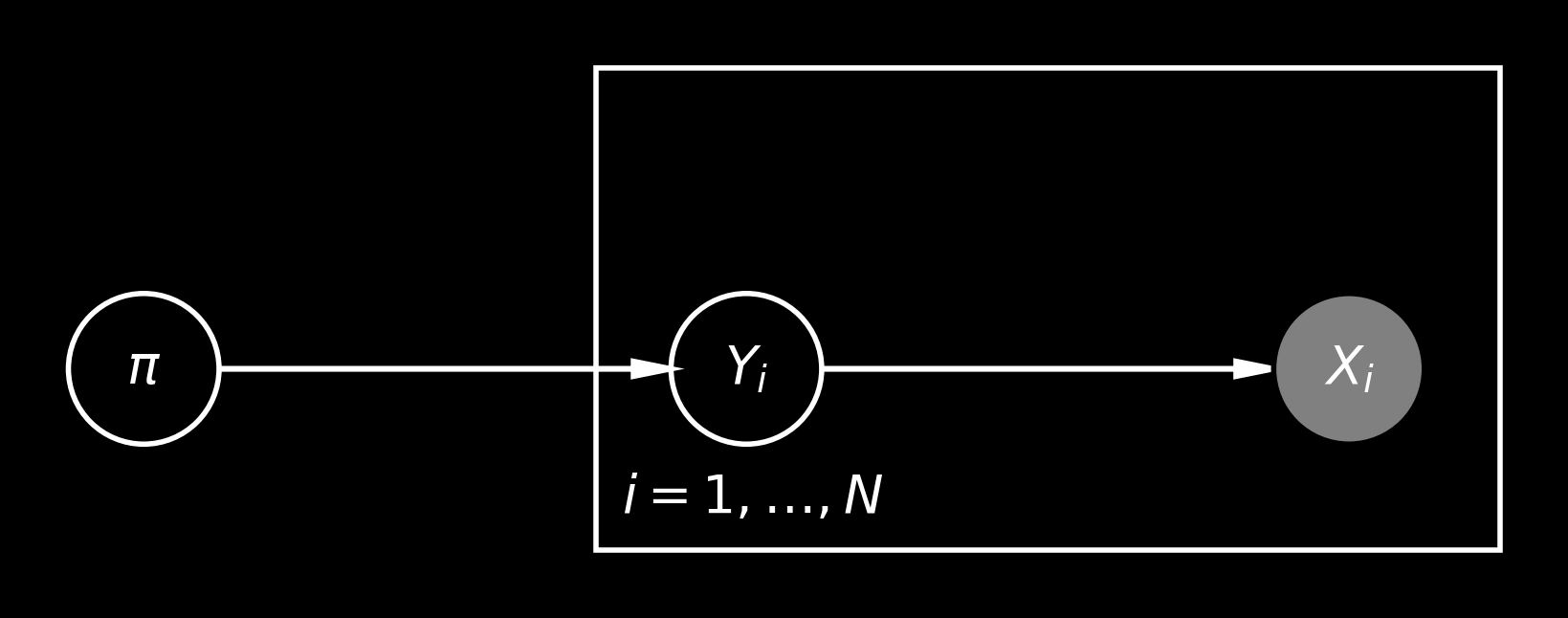
The model is very similar to the one used in clustering problems: for each object we have an observed random variable \(X_i\) (with its realization being the image \(x_i\)) and a latent random variable \(Y_i\), which is valued in the set of labels \(\{1, \dotsc, L\}\).

Additionally, there’s a latent vector \(\pi = (\pi_1, \dotsc, \pi_L)\) with non-negative entries, such that \(\pi_1 + \cdots + \pi_L = 1\). In other words, vector \(\pi\) is the proportion vector of interest.

We can visualise the assumed dependencies in the following graphical model:

Code

import daft
import matplotlib.pyplot as plt
plt.style.use("dark_background")

# Instantiate a PGM object
pgm = daft.PGM(dpi=200)

def add_node(id: str, name: str, x: float, y: float, observed: bool = False):
  if observed:
    params={"facecolor": "grey"}
  else:
    params={"edgecolor": "w"}
  pgm.add_node(id, name, x, y, plot_params=params)

def add_edge(start: str, end: str):
  pgm.add_edge(start, end, plot_params={"edgecolor": "w", "facecolor": "w"})

def add_plate(coords, label: str, shift: float):
  pgm.add_plate(coords, label=label, shift=shift, rect_params={"edgecolor": "w"})

add_node("pi", "$\\pi$", 0, 1)
add_node("Y_i", r"$Y_i$", 2, 1)
add_node("X_i", r"$X_i$", 4, 1, observed=True)

# Add edges
add_edge("pi", "Y_i")
add_edge("Y_i", "X_i")

# Add a plate
add_plate([1.5, 0.5, 3, 1.5], label=r"$i = 1, \ldots, N$", shift=-0.1)

# Render and show the PGM
pgm.render()
plt.show()

As \(\pi\) is simplex-valued, it’s convenient to model it with a Dirichlet prior. Then, \(Y_i\mid \pi \sim \mathrm{Categorical}(\pi)\). Finally, we assume that each class \(y\) has a corresponding distribution \(D_y\) from which the image is sampled. In other words, \(X_i\mid Y_i=y \sim D_y\).

In case we know all distributions \(D_y\), this is quite a simple problem: we can marginalise the latent variables \(Y_i\) obtaining \[ P(\{X_i=x_i\} \mid \pi) = \prod_{i=1}^N \big( \pi_1 D_1(x_i) + \cdots + \pi_L D_L(x_i) \big) \] which in turn can be used to infer \(\pi\) using Hamiltonian Markov chain Monte Carlo algorithms. In fact, a variant of this approach, employing maximum likelihood estimate, rather than Bayesian inference, was proposed by Peters and Coberly (1976) as early as in 1976!

Why expectation-maximization?

However, learning well-calibrated generative models \(D_y\) may be very hard task. Saerens, Latinne, and Decaestecker (2001) instead propose to learn a well-calibrated probabilistic classifier \(P(Y \mid X, \pi^{(0)})\) on an auxiliary population.

The assumption on the auxiliary population is the following: the conditional probability distributions \(D_y = P(X\mid Y=y)\) have to be the same. The only thing that can differ is the proportion vector \(\pi_0\), assumed to be known. This assumption is called prior probability shift or label shift and is rather strong, but also quite hard to avoid: if arbitrary distribution shifts are avoided, it’s not possible to generalize from one distribution to another! Finding suitable ways how to weaken the prior probability shift is therefore an interesting research problem on its own.

Note that if we have a well-calibrated classifier \(P(Y\mid X, \pi^{(0)})\), we also have an access to a distribution \(P(Y\mid X, \pi)\). Namely, note that \[\begin{align*} P(Y=y\mid X=x, \pi) &\propto P(Y=y, X=x \mid \pi) \\ &= P(X=x \mid Y=y, \pi) P(Y=y\mid \pi) \\ &= P(X=x \mid Y=y)\, \pi_y, \end{align*} \] where the proportionality constant does not depend on \(y\). Analogously, \[ P(Y=y\mid X=x, \pi^{(0)}) \propto P(X=x\mid Y=y)\, \pi^{(0)}_y, \] where the key observation is that for both distributions we assume that the conditional distribution \(P(X=x\mid Y=y)\) is the same. Now we can take the ratio of both expressions and obtain \[ P(Y=y\mid X=x, \pi) \propto P(Y=y\mid X=x, \pi^{(0)}) \frac{ \pi_y }{\pi^{(0)}_y}, \] where the proportionality does not depend on \(y\). Hence, we can calculate unnormalized probabilities in this manner and then normalize them, so that they sum up to \(1\).

To summarize, we have the access to:

Well-calibrated probability \(P(Y=y\mid X=x, \pi)\);
The prior probability \(P(\pi)\);
The probability \(P(Y_i=y \mid \pi) = \pi_y\);

and we want to do inference on the posterior \(P(\pi \mid \{X_i\})\).

Expectation-maximization

Expectation-maximization is an iterative algorithm trying to find a stationary point of the log-posterior \[\begin{align*} \log P(\pi \mid \{X_i=x_i\}) &= P(\pi) + \log P(\{X_i = x_i\} \mid \pi) \\ &= P(\pi) + \sum_{i=1}^N \log P(X_i=x_i\mid \pi). \end{align*} \]

In particular, by running the optimization procedure several times, we can hope to find the maximum a posteriori estimate (or the maximum likelihood estimate, when the uniform distribution over the simplex is used as \(P(\pi)\)). Interestingly, this optimization procedure will not assume that we can compute \(\log P(X_i=x_i\mid \pi)\), using instead quantities available to us.

Assume that at the current iteration the proportion vector is \(\pi^{(t)}\). Then, \[\begin{align*} \log P(X_i = x_i\mid \pi) &= \log \sum_{y=1}^L P(X_i = x_i, Y_i = y\mid \pi) \\ &= \log \sum_{y=1}^L P(Y_i=y \mid \pi^{(t)}, X_i = x_i ) \frac{ P(X_i=x_i, Y_i=y \mid \pi) }{P(Y_i=y \mid \pi^{(t)}, X_i=x_i)} \\ &\ge \sum_{y=1}^L P(Y_i=y\mid \pi^{(t)}, X_i=x_i) \log \frac{P(X_i=x_i, Y_i=y \mid \pi)}{P(Y_i=y \mid \pi^{(t)}, X_i=x_i)} \end{align*} \]

where the inequality follows from Jensen’s inequality for concave functions².

We can now bound the loglikelihood by \[\begin{align*} \log P(\{X_i = x_i \}\mid \pi) &= \sum_{i=1}^N \log P(X_i=x_i\mid \pi) \\ &\ge \sum_{i=1}^N \sum_{y=1}^L P(Y_i=y\mid \pi^{(t)}, X_i=x_i) \log \frac{P(X_i=x_i, Y_i=y \mid \pi)}{P(Y_i=y \mid \pi^{(t)}, X_i=x_i)}. \end{align*} \]

Now let \[ Q(\pi, \pi^{(t)}) = \log P(\pi) + \sum_{i=1}^N \sum_{y=1}^L P(Y_i=y\mid \pi^{(t)}, X_i=x_i) \log \frac{P(X_i=x_i, Y_i=y \mid \pi)}{P(Y_i=y \mid \pi^{(t)}, X_i=x_i)}, \] which is a lower bound on the log-posterior. We will define the value \(\pi^{(t+1)}\) by optimizing this lower bound: \[ \pi^{(t+1)} := \mathrm{argmax}_\pi Q(\pi, \pi^{(t)}). \]

Let’s define auxiliary quantities \(\xi_{iy} = P(Y_i=y \mid \pi^{(t)}, X_i=x_i)\), which can be calculated using the probabilistic classifier, as outlined above. This is called the expectation step (although we are actually calculating just probabilities, rather than more general expectations). In the new notation we have \[ Q(\pi, \pi^{(t)}) = \log P(\pi) + \sum_{i=1}^N\sum_{y=1}^L \left(\xi_{iy} \log P(X_i=x_i, Y_i=y\mid \pi) - \xi_{iy} \log \xi_{iy}\right) \]

The term \(\xi_{iy}\log \xi_{iy}\) does not depend on \(\pi\), so we don’t have to include it in the optimization. Writing \(\log P(X_i = x_i, Y_i=y\mid \pi) = \log D_y(x_i) + \log \pi_y\) we see that it suffices to optimize for \(\pi\) the expression \[ \log P(\pi) + \sum_{i=1}^N\sum_{y=1}^L \xi_{iy}\left( \log \pi_y + \log D_y(x_i) \right). \] Even better: not only \(\xi_{iy}\) does not depend on \(\pi\), but also \(\log D_y(x_i)\)! Hence, we can drop from the optimization the terms requiring the generative models and we are left only with the easy to calculate quantities: \[ \log P(\pi) + \sum_{i=1}^N\sum_{y=1}^L \xi_{iy} \log \pi_y. \]

Let’s use the prior \(P(\pi) = \mathrm{Dirichlet}(\pi \mid \alpha_1, \dotsc, \alpha_L)\), so that \(\log P(\pi) = \mathrm{const.} + \sum_{y=1}^L (\alpha_y-1)\log \pi_y\). Hence, we are interested in optimising \[ \sum_{y=1}^L \left((\alpha_y-1) + \sum_{i=1}^N \xi_{iy} \right)\log \pi_y. \]

Write \(A_y = \alpha_y - 1 + \sum_{i=1}^N\xi_{iy}\). We have to optimize the expression \[ \sum_{y=1}^L A_y\log \pi_y \] under a constraint \(\pi_1 + \cdots + \pi_L = 1\).

Saerens, Latinne, and Decaestecker (2001) use Lagrange multipliers, but we will use the first \(L-1\) coordinates to parameterise the simplex and write \(\pi_L = 1 - (\pi_1 + \cdots + \pi_{L-1})\). In this case, if we differentiate with respect to \(\pi_l\), we obtain \[ \frac{A_l}{\pi_l} + \frac{A_L}{\pi_L} \cdot (-1) = 0, \]

which in turn gives that \(\pi_y = k A_y\) for some constant \(k > 0\). We have \[ \sum_{y=1}^L A_y = \sum_{y=1}^L \alpha_y - L + \sum_{i=1}^N\sum_{y=1}^L \xi_{iy} = \sum_{y=1}^L \alpha_y - L + N. \] Hence, \[ \pi_y = \frac{1}{(\alpha_1 + \cdots + \alpha_L) + N - L}\left( \alpha_y-1 + \sum_{i=1}^N \xi_{iy} \right), \] which is taken as the next \(\pi^{(t+1)}\).

As a minor observation, note that for a uniform prior over the simplex (i.e., all \(\alpha_y = 1\)) we have \[ \pi^{(t+1)}_y = \frac 1N\sum_{i=1}^N P(Y_i=y_i \mid X_i=x_i, \pi^{(t)} ). \] Once we have converged to a fixed point and we have \(\pi^{(t)} = \pi^{(t+1)}\), it very much looks like \[ P(Y) = \frac 1N\sum_{i=1}^N P(Y_i \mid X_i, \pi) \approx \mathbb E_{X \sim \pi_1 D_1 + \dotsc + \pi_L D_L}[ P(Y\mid X) ] \] when \(N\) is large.

Gibbs sampler

Finally, let’s think how to implement a Gibbs sampler for this problem. Compared to the expectation-maximization this will be easy.

To solve the quantification problem we have to sample from the posterior distribution \(P(\pi \mid \{X_i\})\). Instead, let’s sample from a high-dimensional distribution \(P(\pi, \{Y_i\} \mid \{X_i\})\) — once we have samples of the form \((\pi, \{Y_i\})\) we can simply forget about the \(Y_i\) values.

This is computationally a harder problem (we have many more variables to sample), however each sampling step will be very convenient. We will alternatively sample from \[ \pi \sim P(\pi \mid \{X_i, Y_i\}) \] and \[ \{Y_i\} \sim P(\{Y_i\} \mid \{X_i\}, \pi). \]

The first step is easy: \(P(\pi \mid \{X_i, Y_i\}) = P(\pi\mid \{Y_i\})\) which (assuming a Dirichlet prior) is a Dirichlet distribution. Namely, if \(P(\pi) = \mathrm{Dirichlet}(\alpha_1, \dotsc, \alpha_L)\), then \[ P(\pi\mid \{Y_i=y_i\}) = \mathrm{Dirichlet}\left( \alpha_1 + \sum_{i=1}^N \mathbf{1}[y_i = 1], \dotsc, \alpha_L + \sum_{i=1}^N \mathbf{1}[y_i=L] \right). \]

Let’s think how to sample \(\{Y_i\} \sim P(\{Y_i\} \mid \{X_i\}, \pi)\). This is a high-dimensional distribution, so let’s… use Gibbs sampling. Namely, we can iteratively sample \[ Y_k \sim P(Y_k \mid \{Y_1, \dotsc, Y_{k-1}, Y_{k+1}, \dotsc, Y_L\}, \{X_i\}, \pi). \]

Thanks to the particular structure of this model, this is equivalent to sampling from \[ Y_k \sim P(Y_k \mid X_k, \pi) = \mathrm{Categorical}(\xi_{k1}, \dotsc, \xi_{kL}), \] where \(\xi_{ky} = P(Y_k = y\mid X_k = x_k, \pi)\) is obtained by recalibrating the given classifier.

Summary

To sum up, the reviewer was right: it’s very simple to upgrade the inference scheme in this model from a point estimate to a sample from the posterior!

I however haven’t run simulations to know how well this sampler works in practice: I expect that this approach could suffer from:

Problems from not-so-well-calibrated probabilistic classifier.
Each iteration of the algorithm (whether expectation-maximization or a Gibbs sampler) requires passing through all \(N\) examples.
As there are \(N\) latent variables sampled, the convergence may perhaps be slow.

It’d be interesting to see how problematic these points are in practice (perhaps not at all!)

Appendix: numerical implementation in JAX

As these algorithms are so simple, let’s quickly implement them in JAX. We will consider two Gaussian densities \(D_1 = \mathcal N(0, 1^2)\) and \(D_2 = \mathcal N(\mu, 1^2)\). Let’s generate some data:

Code

import jax
import jax.numpy as jnp
from jax import random
from jaxtyping import Array, Float, Int
from jax.scipy.special import logsumexp

n_cases: Int[Array, " classes"] = jnp.asarray([10, 40], dtype=int)
mus: Float[Array, " classes"] = jnp.asarray([0.0, 1.0])

key = random.PRNGKey(42)
key, *subkeys = random.split(key, len(n_cases) + 1)

xs: Float[Array, " points"] = jnp.concatenate(tuple(
  mu + random.normal(subkey, shape=(n,))
  for subkey, n, mu in zip(subkeys, n_cases, mus)
))

n_classes: int = len(n_cases)
n_points: int = len(xs)

An NVIDIA GPU may be present on this machine, but a CUDA-enabled jaxlib is not installed. Falling back to cpu.

Now we need a probabilistic classifier. We will assume that it was calibrated on population with proportion \(\pi^{(0)} = (0.4, 0.6)\).

Code

_normalizer: float = 0.5 * jnp.log(2 * jnp.pi)

def log_p(x, mu: float) -> float:
  """Log-density N(x | mu, 1^2)."""
  return -0.5 * jnp.square(x - mu) - _normalizer


# Auxiliary matrix log P(X | Y)
_log_p_x_y: Float[Array, "points classes"] = jnp.stack(tuple(log_p(xs, mu) for mu in mus)).T
assert _log_p_x_y.shape == (n_points, n_classes), f"Shape mismatch: {_log_p_x_y.shape}."

log_pi0: Float[Array, " classes"] = jnp.log(jnp.asarray([0.4, 0.6]))

# Matrix representing log P(Y | X) for labeled population
log_p_y_x: Float[Array, "points classes"] = _log_p_x_y + log_pi0[None, :]
# ... currently it's unnormalized, so we have to normalize it

def normalize_logprobs(log_ps: Float[Array, "points classes"]) -> Float[Array, "points classes"]:
  log_const = logsumexp(log_ps, keepdims=True, axis=-1)
  return log_ps - log_const

log_p_y_x = normalize_logprobs(log_p_y_x)

# Let's quickly check if it works
sums = jnp.sum(jnp.exp(log_p_y_x), axis=1)
assert sums.shape == (n_points,)
assert jnp.min(sums) > 0.999, f"Minimum: {jnp.min(sums)}."
assert jnp.max(sums) < 1.001, f"Maximum: {jnp.max(sums)}."

Expectation-maximization algorithm

It’s time to implement expectation-maximization.

Code

def expectation_maximization(
  log_p_y_x: Float[Array, "points classes"],
  log_pi0: Float[Array, " classes"],
  log_start: None | Float[Array, " classes"] = None,
  alpha: Float[Array, " classes"] | None = None,
  n_iterations: int = 10_000,
) -> Float[Array, " classes"]:
  """Runs the expectation-maximization algorithm.

  Args:
    log_p_y_x: array log P(Y | X) for the calibrated population
    log_pi0: array log P(Y) for the calibrated population
    log_start: starting point. If not provided, `log_pi0` will be used
    alpha: concentration parameters for the Dirichlet prior.
      If not provided, the uniform prior will be used
    n_iterations: number of iterations to run the algorithm for
  """
  if log_start is None:
    log_start = log_pi0
  if alpha is None:
    alpha = jnp.ones_like(log_pi0)

  def iteration(_, log_pi: Float[Array, " classes"]) -> Float[Array, " classes"]:
    # Calculate log xi[n, y]
    log_ps = normalize_logprobs(log_p_y_x + log_pi[None, :] - log_pi0[None, :])
    # Sum xi[n, y] over n. We use the logsumexp, as we have log xi[n, y]
    summed = jnp.exp(logsumexp(log_ps, axis=0, keepdims=False))
    # The term inside the bracket (numerator)
    numerator = summed + alpha - 1.0
    # Denominator
    denominator = jnp.sum(alpha) + log_p_y_x.shape[0] - log_p_y_x.shape[1]
    return jnp.log(numerator / denominator)

  return jax.lax.fori_loop(
    0, n_iterations, iteration, log_start
  )

log_estimated = expectation_maximization(
  log_p_y_x=log_p_y_x,
  log_pi0=log_pi0,
  n_iterations=1000,
  # Let's use slight shrinkage towards more uniform solutions
  alpha=2.0 * jnp.ones_like(log_pi0),
)
estimated = jnp.exp(log_estimated)
print(f"Estimated: {estimated}")
print(f"Actual:    {n_cases / n_cases.sum()}")

Estimated: [0.16425547 0.83574456]
Actual:    [0.2 0.8]

Gibbs sampler

Expectation-maximization returns only a point estimate. We’ll explore the region around the posterior mode with a Gibbs sampler.

Code

def gibbs_sampler(
  key: random.PRNGKeyArray,
  log_p_y_x: Float[Array, "points classes"],
  log_pi0: Float[Array, " classes"],
  log_start: None | Float[Array, " classes"] = None,
  alpha: Float[Array, " classes"] | None = None,
  n_warmup: int = 1_000,
  n_samples: int = 1_000,
) -> Float[Array, "n_samples classes"]:
  if log_start is None:
    log_start = log_pi0
  if alpha is None:
    alpha = jnp.ones_like(log_pi0)

  def iteration(
    log_ps: Float[Array, " classes"],
    key: random.PRNGKeyArray,
  ) -> tuple[Float[Array, " classes"], Float[Array, " classes"]]:
    key, subkey1, subkey2 = random.split(key, 3)

    ys = random.categorical(
      subkey1,
      log_ps[None, :] + log_p_y_x - log_pi0[None, :],
      axis=-1,
    )
    counts = jnp.bincount(ys, length=log_pi0.shape[0])

    new_log_pi = jnp.log(
      random.dirichlet(subkey2, alpha + counts)
    )

    return new_log_pi, new_log_pi

  _, samples = jax.lax.scan(
    iteration,
    log_start,
    random.split(key, n_warmup + n_samples),
  )
  return samples[n_warmup:, :]

key, subkey = random.split(key)
samples = gibbs_sampler(
  key=subkey,
  log_p_y_x=log_p_y_x,
  log_pi0=log_pi0,
  # Let's use slight shrinkage towards more uniform solutions
  alpha=2.0 * jnp.ones_like(log_pi0),
  # Use EM point as a starting point
  log_start=log_estimated,
  n_samples=5_000,
)
samples = jnp.exp(samples)

print(f"Mean:   {jnp.mean(samples, axis=0)}")
print(f"Std:    {jnp.std(samples, axis=0)}")
print(f"Actual: {n_cases / n_cases.sum()}")

/tmp/ipykernel_43705/3942328187.py:2: DeprecationWarning: jax.random.PRNGKeyArray is deprecated. Use jax.Array for annotations, and jax.dtypes.issubdtype(arr.dtype, jax.dtypes.prng_key) for runtime detection of typed prng keys.
  key: random.PRNGKeyArray,
/tmp/ipykernel_43705/3942328187.py:17: DeprecationWarning: jax.random.PRNGKeyArray is deprecated. Use jax.Array for annotations, and jax.dtypes.issubdtype(arr.dtype, jax.dtypes.prng_key) for runtime detection of typed prng keys.
  key: random.PRNGKeyArray,

Mean:   [0.20171012 0.79828984]
Std:    [0.09912279 0.09912279]
Actual: [0.2 0.8]

Let’s visualise the posterior samples, together with the expectation-maximization solution and the ground truth:

Code

import matplotlib.pyplot as plt
plt.style.use("dark_background")

fig, ax = plt.subplots(dpi=150)

bins = jnp.linspace(0, 1, 40)

for y in range(n_classes):
  color = f"C{y+1}"
  ax.hist(samples[:, y], bins=bins, density=True, histtype="step", color=color)
  ax.axvline(n_cases[y] / n_cases.sum(), color=color, linewidth=3)
  ax.axvline(estimated[y], color=color, linestyle="--")

ax.set_title("Posterior distribution")
ax.set_ylabel("Posterior density")
ax.set_xlabel("Component value")
ax.spines[["top", "right"]].set_visible(False)
fig.tight_layout()

References

Peters, C., and W. A Coberly. 1976. “The Numerical Evaluation of the Maximum-Likelihood Estimate of Mixture Proportions.” Communications in Statistics – Theory and Methods 5: 1127–35.

Saerens, Marco, Patrice Latinne, and Christine Decaestecker. 2001. “Adjusting the Outputs of a Classifier to New a Priori Probabilities: A Simple Procedure.” Neural Computation 14: 14–21.

Ziegler, Albert, and Paweł Czyż. 2023. “Bayesian Quantification with Black-Box Estimators.” https://arxiv.org/abs/2302.09159.

Footnotes

Let’s call this problem “quantification of uncertainty in quantification problems”.↩︎
It’s good to remember: \(\log \mathbb E[A] \ge \mathbb E[\log A]\).↩︎