From \(t\)-test to “This is what ‘power=0.06’ looks like”

We take a close look at the derivation of the \(t\)-test and reproduce plots used by Andrew Gelman to show implications of low-powered studies.

Andrew Gelman wrote an amazing blogpost, where he argues that with large noise-to-signal ratio (low power studies) statistically significant results:

• Often have exagerrated effect size.
• Have large chance of being the wrong sign. Art Owen made an additional plot demonstrating this effect.

This is especially troublesome because as there is a tradition of publishing only statistically significant results¹, many of the reported effects will have the wrong sign or be seriously exaggerated.

But we’ll take a look at these phenomena later. First, let’s review what the \(t\)-test, confidence intervals, and statistical power are.

A quick overview of \(t\)-test

Recall that if we have access to i.i.d. random variables
\[ X_1, \dotsc, X_n \sim \mathcal N(\mu, \sigma^2), \] we introduce sample mean \[ M = \frac{X_1 + \cdots + X_n}{n} \] and sample standard deviation: \[ S = \sqrt{ \frac{1}{n-1} \sum_{i=1}^n \left(X_i - M\right)^2}. \]

It follows that \[ M\sim \mathcal N(\mu, \sigma^2/n) \] and \[ S^2\cdot (n-1)/\sigma^2 \sim \chi^2_{n-1} \] are independent. We can construct a pivot \[ T_\mu = \frac{M-\mu}{S / \sqrt{n}}, \] which is distributed according to Student’s \(t\) distribution² with \(n-1\) degrees of freedom, \(t_{n-1}\).

Choose a number \(0 < \alpha < 1\) and write \(u\) for the solution to the equation \[ P(T_\mu \in (-u, u)) = 1-\alpha. \]

The \(t\) distribution is continuous and symmetric around \(0\), so that \[ \mathrm{CDF}(-u) = 1 - \mathrm{CDF}(u) \] and \[ P(T_\mu \in (-u, u)) = \mathrm{CDF}(u) - \mathrm{CDF}(-u) = 2\cdot \mathrm{CDF}(u) - 1. \]

From this we have \[ \mathrm{CDF}(u) = 1 - \alpha / 2. \]

Hence, we have \[ P(\mu \in ( M - \delta, M + \delta )) = 1 - \alpha, \] where \[ \delta = u \cdot\frac{S}{\sqrt{n}} \] is the half-width of the confidence interval.

In this way we have constructed a confidence interval with coverage \(1-\alpha\). Note that \(u\) coresponds to the \((1-\alpha/2)\)th quantile. For example, if we want coverage of \(95\%\), we take \(\alpha=5\%\) and \(u\) will be the 97.5th percentile.

Hypothesis testing

Consider a hypothesis \(H_0\colon \mu = 0\).

We will reject \(H_0\) if \(0\) is outside of the confidence interval defined above. Note that \[ P( 0 \in (M-\delta, M + \delta) \mid H_0 ) = 1-\alpha \] and \[ P(0 \not\in (M-\delta, M + \delta) \mid H_0 ) = 1 - (1-\alpha) = \alpha, \] meaning that such a test will have false discovery rate \(\alpha\).

Interlude: \(p\)-values

The above test is often presented in terms of \(p\)-values. Define the \(t\)-statistic \[ T_0 = \frac{M}{S/\sqrt{n}}, \] which does not require the knowledge of a true \(\mu\). Note that if \(H_0\) is true, then \(T_0\) will be distributed according to \(t_{n-1}\) distribution. (If \(H_0\) is false, then it won’t be. We will take a closer look at this case when we discuss power).

We have \(T_0 \in (-u, u)\) if and only if \(0\) is inside the confidence interval defined above: we can reject \(H_0\) whenever \(|T_0| \ge u\). As the procedure hasn’t really changed, we also have \[ P(T_0 \in (-u, u) \mid H_0 ) = P( |T_0| < u \mid H_0 ) = 1-\alpha \] and this test again has false discovery rate \(\alpha\).

Now define \[ \Pi = 2\cdot (1 - \mathrm{CDF}( |T_0| ) ) = 2\cdot \mathrm{CDF}(-|T_0|). \] Note that we have

\[\begin{align*} \Pi < \alpha &\Leftrightarrow 2\cdot (1-\mathrm{CDF}(|T_0|)) < 2\cdot (1-\mathrm{CDF}(u)) \\ &\Leftrightarrow 1- \mathrm{CDF}(|T_0|) < 1 - \mathrm{CDF}(u) \\ &\Leftrightarrow \mathrm{CDF}(-|T_0|) < \mathrm{CDF}(-u)\\ &\Leftrightarrow -|T_0| < -u \\ &\Leftrightarrow |T_0| > u, \end{align*} \]

so that we can compare the \(p\)-value \(\Pi\) against false discovery rate \(\alpha\).

Both comparisons are equivalent and equally hard to compute: the hard part of comparing \(|T_0|\) against \(u\) is calculation of \(u\) from \(\alpha\) (which requires the access to the CDF). The hard part of comparing the \(p\)-value \(\Pi\) against \(\alpha\) is calculation of \(\Pi\) from \(|T_0|\) (which requires the access to the CDF). I should also add that, as we will see below, the CDF is actually easy to access in Python.

Let’s also observe that we have \[ P( \Pi \le \alpha \mid H_0 ) = P( |T_0| \ge u \mid H_0 ) = \alpha, \] meaning that if the null hypothesis is true, then \(\Pi\) has the uniform distribution over the interval \((0, 1)\).

Summary

• Choose a coverage level \(1-\alpha\).
• Collect a sample of size \(n\).
• Calculate \(u\) as using \(\mathrm{CDF}(u)=1-\alpha/2\), or equivalently, \(\alpha = 2\cdot ( 1 - \mathrm{CDF}(u) )\), where we use the CDF of the Student distribution with \(n-1\) degrees of freedom.
• Calculate sample mean and sample standard deviation, \(M\) and \(S\).
• Construct the confidence interval as \(M\pm uS/\sqrt{n}\).
• To test for \(H_0\colon \mu = 0\) check if \(\mu_0\) is outside of the confidence interval (to reject \(H_0\)).
• Alternatively, construct \(T_0 = M\sqrt{n}/S\) and compare \(|T_0| > u\) (to reject \(H_0\)).
• Alternatively, construct \(\Pi = 2\cdot (1-\mathrm{CDF}(|T_0|))\) and check whether \(\Pi < \alpha\) (to reject \(H_0\)).

A bit of code

Let’s implement the above formulae using SciPy’s \(t\) distribution to keep things as related to the formulae above as possible. Any discrepancies will suggest an error in the derivations or a bug in the code.

Code

import numpy as np

from scipy import stats

def alpha_to_u(alpha: float, nobs: int) -> float:
  if np.min(alpha) <= 0 or np.max(alpha) >= 1:
    raise ValueError("Alpha has to be inside (0, 1).")
  return stats.t.ppf(1 - alpha / 2, df=nobs - 1)


def u_to_alpha(u: float, nobs: int) -> float:
  if np.min(u) <= 0:
    raise ValueError("u has to be positive")
  return 2 * (1 - stats.t.cdf(u, df=nobs - 1))

# Let's test whether the functions seem to be compatible
for alpha in [0.01, 0.05, 0.1, 0.99]:
  for nobs in [5, 10]:
    u = alpha_to_u(alpha, nobs=nobs)
    a = u_to_alpha(u, nobs=nobs)

    if abs(a - alpha) > 1e-4:
      raise ValueError(f"Discrepancy for {nobs=} {alpha=}")


def calculate_t(xs: np.ndarray):
  # Sample mean and sample standard deviation
  n = len(xs)
  m = np.mean(xs)
  s = np.std(xs, ddof=1)

  # Calculate the t value assuming the null hypothesis mu = 0
  t = m / (s / np.sqrt(n))
  return t

def calculate_p_value_from_t(t: float, nobs: int) -> float:
  return 2 * (1 - stats.t.cdf(np.abs(t), df=nobs-1))

def calculate_p_value_from_data(xs: np.ndarray) -> float:
  n = len(xs)
  t = calculate_t(xs)
  return calculate_p_value_from_t(t=t, nobs=n)

def calculate_ci_delta_from_params(
  s: float,
  nobs: int,
  alpha: float,
) -> tuple[float, float]:
  u = alpha_to_u(alpha, nobs=nobs)
  delta = u * s / np.sqrt(nobs)
  return delta

def calculate_ci_delta_from_data(xs: np.ndarray, alpha: float) -> float:
  m = np.mean(xs)
  s = np.std(xs, ddof=1)
  delta = calculate_ci_delta_from_params(s=s, nobs=len(xs), alpha=alpha)
  return delta

def calculate_confidence_interval_from_data(
  xs: np.ndarray,
  alpha: float,
) -> tuple[float, float]:
  delta = calculate_ci_delta_from_data(xs, alpha=alpha)
  return (m-delta, m+delta)

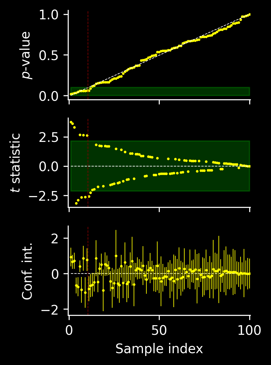
We have three equivalent tests for rejecting \(H_0\). Let’s see how they perform on several samples. We’ll simulate \(N\) times a fresh data set \(X_1, \dotsc, X_n\) from \(\mathcal N\left(0, \sigma^2\right)\) and calculate the confidence interval, the \(T_0\) statistic and the \(p\)-value for each of these. We will order the samples by increasing \(p\)-value (equivalently, with decreasing \(|T_0|\) statistic), to make dependencies in the plot easier to see.

Additionally, we will choose relatively large \(\alpha\) and mark the regions such that the test does not reject \(H_0\). In terms of confidence intervals there is no such region, as each sample which has its own confidence interval, which can contain \(0\) or not.

Code

import matplotlib.pyplot as plt
plt.style.use("dark_background")

rng = np.random.default_rng(42)

nsimul = 100
nobs = 5

samples = rng.normal(loc=0, scale=1.0, size=(nsimul, nobs))
p_values = np.asarray([calculate_p_value_from_data(x) for x in samples])
index = np.argsort(p_values)


alpha: float = 0.1
u_thresh = alpha_to_u(alpha, nobs=nobs)

samples = samples[index, :]
p_values = p_values[index]
t_stats = np.asarray([calculate_t(x) for x in samples])
sample_means = np.mean(samples, axis=1)
ci_deltas = np.asarray([calculate_ci_delta_from_data(x, alpha=alpha) for x in samples])

x_axis = np.arange(1, nsimul + 1)
fig, axs = plt.subplots(3, 1, figsize=(3, 4), dpi=150, sharex=True)

# P-values plot
ax = axs[0]
ax.fill_between(x_axis, alpha, 0, color="lime", alpha=0.2)
ax.plot(x_axis, np.linspace(0, 1, num=len(x_axis)), linestyle="--", linewidth=0.5, color="white")
ax.scatter(x_axis, p_values, c="yellow", s=1)
ax.set_xlim(-0.5, nsimul + 0.5)
ax.set_ylabel("$p$-value")

ax.axvline(alpha * nsimul + 0.5, color="maroon", linestyle="--", linewidth=0.5)

# T statistics
ax = axs[1]
ax.fill_between(x_axis, -u_thresh, u_thresh, color="lime", alpha=0.2)
ax.scatter(x_axis, t_stats, c="yellow", s=1)
ax.plot(x_axis, np.zeros_like(x_axis), c="white", linestyle="--", linewidth=0.5)
ax.set_ylabel("$t$ statistic")

ax.axvline(alpha * nsimul + 0.5, color="maroon", linestyle="--", linewidth=0.5)

# Confidence intervals
ax = axs[2]
ax.set_xlabel("Sample index")
ax.plot(x_axis, np.zeros_like(x_axis), c="white", linestyle="--", linewidth=0.5)
ax.errorbar(x_axis, sample_means, yerr=ci_deltas, fmt="o", markersize=1, linewidth=0.5, c="yellow")
ax.set_ylabel("Conf. int.")

ax.axvline(alpha * nsimul + 0.5, color="maroon", linestyle="--", linewidth=0.5)

for ax in axs:
  ax.spines[['top', 'right']].set_visible(False)

fig.tight_layout()

Let’s also quickly verify that, indeed, the distribution of \(p\)-values is uniform over \((0, 1)\) (which, in a way, can be already deduced from the plot with ordered \(p\) values) and that the distribution of the \(t\) statistic is indeed \(t_{n-1}\).

Code

fig, axs = plt.subplots(1, 3, figsize=(5, 2), dpi=150)

ax = axs[0]
ax.set_title("CDF ($p$-value)")
x_ax = np.linspace(0, 1, 5)
ax.plot(x_ax, x_ax, color="white", linestyle="--", linewidth=1)
ax.ecdf(p_values, c="maroon")

ax = axs[1]
ax.set_title("CDF ($t$-stat.)")
x_ax = np.linspace(-3.5, 3.5, 101)
ax.plot(x_ax, stats.t.cdf(x_ax, df=nobs-1), color="white", linestyle="--", linewidth=1)
ax.ecdf(t_stats, c="maroon")

ax = axs[2]
ax.set_title("CDF (mean)")
x_ax = np.linspace(-1.2, 1.2, 101)
ax.plot(x_ax, stats.norm.cdf(x_ax, scale=1/np.sqrt(nobs)), color="white", linestyle="--", linewidth=1)
ax.ecdf(sample_means, c="maroon")

for ax in axs:
  ax.spines[['top', 'right']].set_visible(False)

fig.tight_layout()

Statistical power

Above we have seen a procedure used to reject the null hypothesis \(H_0\colon \mu = 0\) either by constructing the confidence interval or defining the variable \(T_0\) with the property that \(P( |T_0| > u \mid H_0) = \alpha.\)

Consider now the data coming from a distribution with any other \(\mu\), i.e., we will not condition on \(H_0\) anymore. To make this explicit in the notation, we will condition on \(H_\mu\), rather than \(H_0\).

How does the distribution of \(T_0\) look like now? Recall that have independent variables \[ \frac{M-\mu}{\sigma/\sqrt{n}} \sim \mathcal N(0, 1) \] and \[ S^2\cdot (n-1)/\sigma^2 \sim \chi^2_{n-1} \] so that we have, of course, \[ T_\mu = \frac{M-\mu}{S/\sqrt{n}} = \frac{ \frac{M-\mu}{\sigma/\sqrt{n}}}{\sqrt{ \frac{ S^2\cdot (n-1)/\sigma^2 }{n-1} }} \sim t_{n-1}. \] For \(T_0\) we have \[ T_0 = \frac{ \frac{M-\mu}{\sigma/\sqrt{n}} + \frac{\mu}{\sigma/\sqrt{n}}}{\sqrt{ \frac{ S^2\cdot (n-1)/\sigma^2 }{n-1} }} \] which is distributed according to the noncentral \(t\) distribution with noncentrality parameter \(\theta = \mu\sqrt{n} / \sigma\). Note that this distribution is generally asymmetric and different from the location-scale generalisation of the (central) \(t\) distribution. Let’s write \(F_{n-1, \theta}\) for the CDF of this function. We will reject the null hypothesis \(H_0\) with probability \[\begin{align*} P(|T_0| > u \mid H_\mu) &= P(T_0 > u \mid H_\mu ) + P(T_0 < -u \mid H_\mu) \\ &= 1 - P(T_0 < u \mid H_\mu) + P(T_0 < -u \mid H_\mu) \\ &= 1 - F_{n-1,\theta}(u) + F_{n-1,\theta}(-u), \end{align*} \]

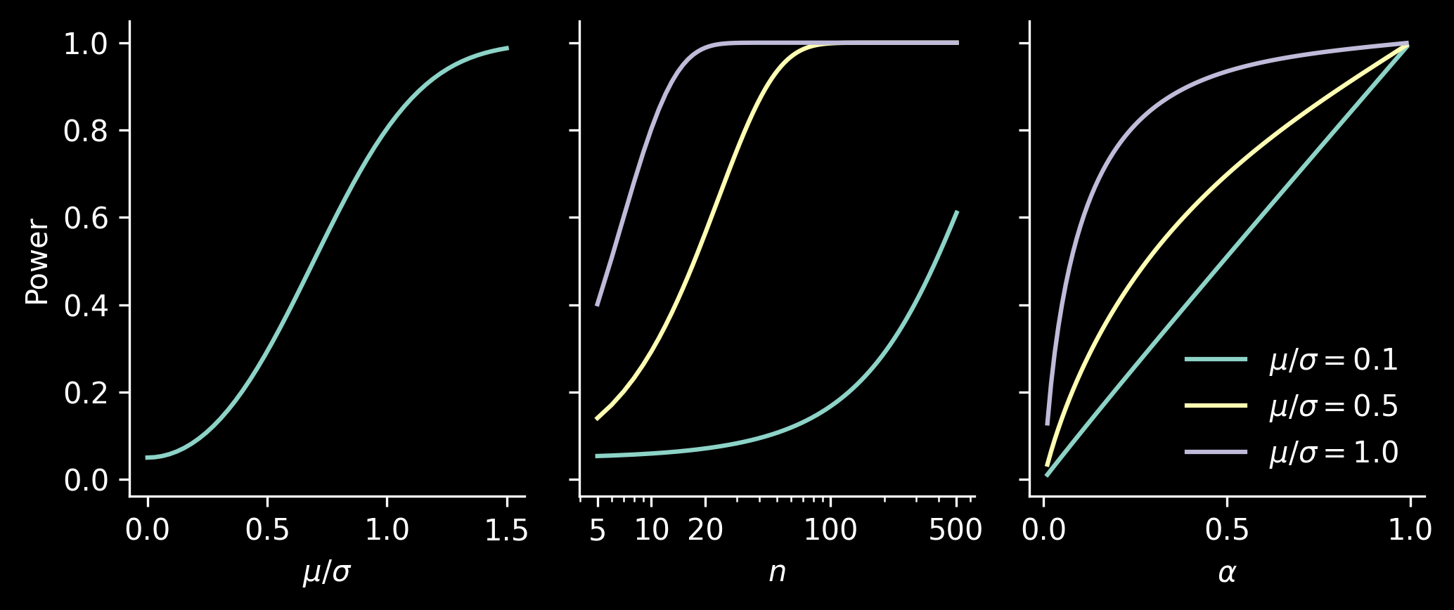
which gives us statistical power of the test.

We see that power depends on chosen \(\alpha\) (as it controls \(u\), the value we compare against the \(|T_0|\) statistic), on \(n\) (as it controls both the number of degrees of freedom in the CDF \(F_{n-1,\theta}\) and the noncentrality parameter \(\theta\)) and on the effect size, by which we understand the standardized mean difference, i.e., \(\mu/\sigma\).

Another bit of code

Let’s implement power calculation. In fact, statsmodels has very convenient utilities for power calculation, so in practice implementing it is never needed:

Code

from statsmodels.stats.power import TTestPower

def calculate_power(
  effect_size: float,
  nobs: int,
  alpha: float,
) -> float:
  theta = np.sqrt(nobs) * effect_size
  u = alpha_to_u(alpha, nobs=nobs)

  def cdf(x: float) -> float:
    return stats.nct.cdf(x, df=nobs-1, nc=theta)
  
  return 1 - cdf(u) + cdf(-u)

for nobs in [5, 10]:
  for alpha in [0.01, 0.05, 0.1]:
    for effect_size in [0, 0.1, 1.0, 3.0]:
      power = calculate_power(
        effect_size=effect_size, nobs=nobs, alpha=alpha,
      )
      power_ = TTestPower().power(
        effect_size=effect_size, nobs=nobs, alpha=alpha, alternative="two-sided")
      
      if abs(power - power_) > 0.001:
        raise ValueError(f"For {nobs=} {alpha=} {effect_size=} we noted discrepancy {power} != {power_}")

Let’s quickly check how power depends on the effect size in the following setting. We collect \(X_1, \dotsc, X_n\sim \mathcal N(\mu, 1^2)\), so that standardized mean difference is \(\mu = \mu/1\) and we will use standard \(\alpha = 5\%\).

Code

fig, axs = plt.subplots(1, 3, figsize=(7, 3), dpi=150, sharey=True)

ax = axs[0]
mus = np.linspace(0, 1.5)
ax.plot(
  mus, calculate_power(effect_size=mus, nobs=10, alpha=0.05)
)
ax.set_xlabel(r"$\mu/\sigma$")
ax.set_ylabel("Power")

ax = axs[1]
ns = np.arange(5, 505)
for eff in [0.1, 0.5, 1.0]:
  ax.plot(
    ns, calculate_power(effect_size=eff, nobs=ns, alpha=0.05),
    label=f"$\mu/\sigma={eff:.1f}$"
  )
ax.set_xscale("log")
n_labels = np.asarray([5, 10, 20, 100, 500])
ax.set_xticks(n_labels, n_labels)
ax.set_xlabel("$n$")

ax = axs[2]
alphas = np.linspace(0.01, 0.99, 99)
for eff in [0.1, 0.5, 1.0]:
  ax.plot(
    alphas, calculate_power(effect_size=eff, nobs=5, alpha=alphas),
    label=f"$\mu/\sigma={eff:.1f}$"
  )
ax.legend(frameon=False)
ax.set_xlabel(r"$\alpha$")

for ax in axs:
  ax.spines[['top', 'right']].set_visible(False)

fig.tight_layout()

/home/pawel/micromamba/envs/data-science/lib/python3.10/site-packages/scipy/stats/_continuous_distns.py:7313: RuntimeWarning: invalid value encountered in _nct_cdf
  return np.clip(_boost._nct_cdf(x, df, nc), 0, 1)

Consequences of low power

Consider a study with \(\sigma=1\), \(\mu=0.1\) and \(n=10\). At \(\alpha = 5\%\) we have power of:

Code

power = calculate_power(effect_size=0.1, nobs=10, alpha=0.05)
if abs(power - 0.06) > 0.005:
  raise ValueError(f"We want power to be around 6%")
print(f"Power: {100 * power:.2f}%")

Power: 5.93%

which is similar to the value used in Andrew Gelman’s post. Let’s simulate a lot of data sets and confirm that the power of the test is indeed around 6%:

Code

nsimul = 200_000
nobs = 10
alpha = 0.05

true_mean = 0.1

samples = rng.normal(loc=true_mean, scale=1.0, size=(nsimul, nobs))
p_values = np.asarray([calculate_p_value_from_data(x) for x in samples])

print(f"Power from simulation: {100 * np.mean(p_values < alpha):.2f}%")

Power from simulation: 5.97%

(As a side note, I already regret not implementing \(p\)-value calculation in JAX – I can’t use vmap!)

Code

fig, axs = plt.subplots(1, 2, figsize=(5, 2), dpi=150, sharex=True)

bins = np.linspace(-1.5, 1.5, 31)

ax = axs[0]
sample_means = np.mean(samples, axis=1)
ax.hist(
  sample_means,
  bins=bins,
  histtype="step",
)
ax.axvline(true_mean)
ax.set_title("Histogram of sample means")
ax.set_xlabel("Sample mean")
ax.set_ylabel("PDF")

ax = axs[1]
x_ax = np.linspace(-1.5, 1.5, 51)
ax.plot(
  x_ax, stats.norm.cdf(x_ax, loc=0.1, scale=1/np.sqrt(nobs))
)
ax.ecdf(sample_means)
ax.set_xlabel("Sample mean")
ax.set_ylabel("CDF")
ax.set_title("Empirical CDF")

for ax in axs:
  ax.spines[['top', 'right']].set_visible(False)

fig.tight_layout()

We see that sample mean, represented by the random variable \(M\), is indeed distributed according to \(\mathcal N\left(0.1, \left(1/\sqrt{10}\right)^2\right)\). The standard error of the mean, \(1/\sqrt{10}\approx 0.31\) is three times larger than the population mean \(\mu=0.1\), so we have a lot of noise here.

Let’s see what happens if a “statistically significant” result is somehow obtained.

Code

stat_signif_samples = samples[p_values < alpha, :]

fig, ax = plt.subplots(figsize=(2, 2), dpi=150)

sample_means = np.mean(stat_signif_samples, axis=1)
ax.hist(
  sample_means,
  bins=bins,
  histtype="step",
)
ax.axvline(true_mean)
ax.set_title("Stat. signif. results")
ax.set_xlabel("Sample mean")
ax.set_ylabel("PDF")


ax.spines[['top', 'right']].set_visible(False)
fig.tight_layout()

Conditioning only on statistically significant results, let’s take a look at:

• how many of them have sample mean of wrong sign,
• how many of them have sample mean seriously exaggerated (e.g., at least 5 times),

similarly as Andrew Gelman did in his blog post:

Code

frac_wrong_sign = np.mean(sample_means < 0)
print(f"Wrong sign: {100*frac_wrong_sign:.1f}%")

frac_exaggerated = np.mean(sample_means >= 5 * true_mean)
print(f"Exaggerated (5x): {100 * frac_exaggerated:.1f}%")

Wrong sign: 20.8%
Exaggerated (5x): 69.5%

Oh, that’s not good! We see that a statistically significant result (which itself has only 6% occurrence probability, if the study is executed properly), will have about 20% chance of being of a wrong sign and around 2/3 chance of being quite exaggerated.

Actually, Andrew Gelman looked at results exaggerated 9 times. Let’s make a plot summarizing these probabilities:

Code

fig, ax = plt.subplots(figsize=(2, 2), dpi=150)

ratio_exag = np.linspace(1, 11, 31)
frac_exag = [np.mean(sample_means >= r * true_mean) for r in ratio_exag]

ax.plot(
  ratio_exag,
  frac_exag,
)
ax.set_ylim(0, 1)
ax.set_xlabel("Exag. factor")
ax.set_ylabel("Probability")
xticks = [1, 3, 5, 7, 9]
ax.set_xticks(xticks, xticks)

ax.spines[['top', 'right']].set_visible(False)
fig.tight_layout()

Finally, there is a great plot by Art Owen showing how confidence intervals of statistically significant results look like when power is low. Let’s quickly reproduce it:

Code

ci_deltas = np.asarray([calculate_ci_delta_from_data(x, alpha=alpha) for x in stat_signif_samples])

n_to_plot = min(50, len(stat_signif_samples))

x_axis = np.arange(1, n_to_plot + 1)
fig, ax = plt.subplots(1, figsize=(3, 2), dpi=150)

ax.set_xlabel("Sample index")

ax.plot(x_axis, np.zeros_like(x_axis), c="white", linestyle="--", linewidth=0.5)
ax.plot(x_axis, np.zeros_like(x_axis) + true_mean, c="maroon", linestyle="-", linewidth=0.5)

ax.errorbar(x_axis, sample_means[:n_to_plot], yerr=ci_deltas[:n_to_plot], fmt="o", markersize=1, linewidth=0.5, c="yellow")
ax.set_ylabel("Conf. int.")

ax.spines[['top', 'right']].set_visible(False)
fig.tight_layout()

Of course, the confidence intervals cannot contain \(0\) (otherwise the results wouldn’t have been statistically significant). How many of them contain \(\mu=0.1\)? In case we look at all the results (including the majority of nonsignificant results), \(1-\alpha=95\%\) of confidence intervals contains the true value. However, once we restrict our attention to only significant results, this coverage drops to

Code

frac_contain = np.mean(
  (sample_means - ci_deltas < true_mean) 
  & (true_mean < sample_means + ci_deltas)
)
print(f"Coverage: {100 * frac_contain:.1f}%")

Coverage: 37.2%

Summary

Low-powered studies have, of course, high probability of not rejecting \(H_0\) when the alternative is true. But even when \(H_0\) is rejected, estimated mean will be often of wring sign or exaggerated. This indeed shows that principled experimental design and power analysis are crucial to execute before any data collection!

Footnotes

1. A practice, which can result in p-hacking and HARKing. On a related manner see this post on negative results and the paper on “the garden of forking paths”.

2. Student’s \(t\) distribution with \(k\) degrees of freedom arises as the distribution of the variable \(T = A/\sqrt{B / k}\), where \(A\sim \mathcal N(0, 1)\) and \(B\sim \chi^2_k\) are independent. In this case, \(\frac{M-\mu}{\sigma/\sqrt{n}}\sim N(0, 1)\) and \(S^2\cdot (n-1)/ \sigma^2 \sim \chi^2_{n-1}\) are independent. Parameter \(\sigma\) cancels out.