Two distributions on a triangle

Sometimes if you misunderstand something, you can have two interesting distributions, rather than only one.

Frederic, Alex and I have been discussing some experiments related to our work on mutual information estimators and Frederic suggested to look at one distribution. I misunderstood what he meant, but this mistake turned out to be quite an interesting object.

So let’s take a look at two distributions defined over a triangle \[T = \{ (x, y)\in (0, 1)\times (0, 1) \mid y < x \}\] and calculate their mutual information.

Uniform joint

Consider a probability distribution with constant probability density function (PDF) of the joint distribution: \[p_{XY}(x, y) = 2 \cdot \mathbf{1}[y<x].\]

We have \[p_X(x) = \int\limits_0^x p_{XY}(x, y)\, \mathrm{d}y = 2x\] and \[ p_Y(y) = \int\limits_0^1 p_{XY}(x, y) \mathbf{1}[y < x] \, \mathrm{d}x = \int\limits_y^1 p_{XY}(x, y) \, \mathrm{d}x = 2(1-y).\]

Hence, pointwise mutual information is given by \[ i(x, y) = \log \frac{ p_{XY}(x, y) }{p_X(x) \, p_Y(y) } = \log \frac{1}{2x(1-y)}\] and mutual information is

\[I(X; Y) = \int\limits_0^1 \mathrm{d}x \int\limits_x^1 i(x, y)\, p_{XY}(x, y) \mathrm{d}y = 1-\log 2 \approx 0.307.\]

Finally, let’s visualise this distribution to numerically validate the formulae above:

Code

from typing import Protocol

import matplotlib.pyplot as plt
import numpy as np

plt.style.use("dark_background")


class Distribution(Protocol):
  def sample(self, rng, n_samples: int) -> np.ndarray:
    pass

  def p_xy(self, x: np.ndarray, y: np.ndarray) -> np.ndarray:
    pass

  def p_x(self, x: np.ndarray) -> np.ndarray:
    pass

  def p_y(self, y: np.ndarray) -> np.ndarray:
    pass

  def pmi(self, x: np.ndarray, y: np.ndarray) -> np.ndarray:
    pass

  @property
  def mi(self) -> float:
    pass


class UniformJoint(Distribution):
  def sample(self, rng, n_samples):
    samples = rng.uniform(low=1e-9, size=(3 * n_samples, 2))
    samples = np.asarray(list(filter(lambda point: point[1] < point[0], samples)))
    if len(samples) < n_samples:
      samples = self.sample(rng, n_samples)
    
    assert len(samples) >= n_samples
    return samples[:n_samples, ...]

  def p_xy(self, x, y):
    return np.where(y < x, 2.0, 0.0)

  def p_x(self, x):
    return 2*x

  def p_y(self, y):
    return 2*(1-y)

  def pmi(self, x, y):
    return np.where(y < x, -np.log(2*x*(1-y)), np.nan)

  @property
  def mi(self):
    return 0.307


def visualise_dist(
  rng,
  dist: Distribution,
  n_samples: int = 15_000,
) -> plt.Figure:
  fig, axs = plt.subplots(2, 3, figsize=(3*2.2, 2*2.2))

  samples = dist.sample(rng, n_samples=n_samples)

  t_axis = np.linspace(1e-9, 1 - 1e-9, 51)

  X, Y = np.meshgrid(t_axis, t_axis)

  # Visualise joint probability
  ax = axs[0, 0]
  ax.scatter(samples[:, 0], samples[:, 1], rasterized=True, alpha=0.3, s=0.2, marker=".")
  ax.set_xlim(0, 1)
  ax.set_ylim(0, 1)
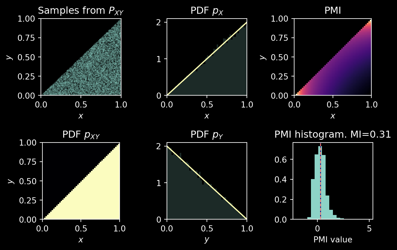
  ax.set_title("Samples from $P_{XY}$")
  ax.set_xlabel("$x$")
  ax.set_ylabel("$y$")

  ax = axs[1, 0]
  ax.imshow(dist.p_xy(X, Y), origin="lower", extent=[0, 1, 0, 1], cmap="magma")
  ax.set_title("PDF $p_{XY}$")
  ax.set_xlabel("$x$")
  ax.set_ylabel("$y$")

  # Visualise marginal distributions
  ax = axs[0, 1]
  ax.set_xlim(0, 1)
  ax.hist(samples[:, 0], bins=np.linspace(0, 1, 51), density=True, alpha=0.2, rasterized=True)
  ax.plot(t_axis, dist.p_x(t_axis))
  ax.set_xlabel("$x$")
  ax.set_title("PDF $p_X$")

  ax = axs[1, 1]
  ax.set_xlim(0, 1)
  ax.hist(samples[:, 1], bins=np.linspace(0, 1, 51), density=True, alpha=0.2, rasterized=True)
  t_axis = np.linspace(0, 1, 51)
  ax.plot(t_axis, dist.p_y(t_axis))
  ax.set_xlabel("$y$")
  ax.set_title("PDF $p_Y$")

  # Visualise PMI
  ax = axs[0, 2]
  ax.set_xlim(0, 1)
  ax.set_ylim(0, 1)
  ax.imshow(dist.pmi(X, Y), origin="lower", extent=[0, 1, 0, 1], cmap="magma")
  ax.set_title("PMI")
  ax.set_xlabel("$x$")
  ax.set_ylabel("$y$")

  ax = axs[1, 2]
  pmi_profile = dist.pmi(samples[:, 0], samples[:, 1])
  mi = np.mean(pmi_profile)
  ax.set_title(f"PMI histogram. MI={dist.mi:.2f}")  
  ax.axvline(mi, color="navy", linewidth=1)
  ax.axvline(dist.mi, color="salmon", linewidth=1, linestyle="--")
  ax.hist(pmi_profile, bins=np.linspace(-2, 5, 21), density=True)
  ax.set_xlabel("PMI value")

  return fig

rng = np.random.default_rng(42)
dist = UniformJoint()

fig = visualise_dist(rng, dist)
fig.tight_layout()

Uniform margin

The above distribution is interesting, but when I heard about the distribution over the triangle, I actually had the following generative model in mind: \[\begin{align*} X &\sim \mathrm{Uniform}(0, 1),\\ Y \mid X=x &\sim \mathrm{Uniform}(0, x). \end{align*}\]

We have \(p_X(x) = 1\) and therefore \[p_{XY}(x, y) = p_{Y\mid X}(y\mid x) = \frac{1}{x}\,\mathbf{1}[y < x].\]

Again, this distribution is defined on the triangle \(T\), although now the joint is not uniform.

We have \[ p_Y(y) = \int\limits_y^1 \frac{1}{x} \, \mathrm{d}x = -\log y\] and \[i(x, y) = \log \frac{1}{-x \log y} = -\log \big(x\cdot (-\log y)\big ) = - \left(\log(x) + \log(-\log y) \right) = -\log x - \log(-\log y).\] This expression suggests that if \(p_Y(y)\) were uniform on \((0, 1)\) (but it is not), the pointwise mutual information \(i(x, Y)\) would be distributed according to Gumbel distribution.

The mutual information \[ I(X; Y) = -\int\limits_0^1 \mathrm{d}y \int\limits_y^1 \frac{ \log x + \log(-\log y)}{x} \, \mathrm{d}x = \frac{1}{2} \int\limits_0^1 \log y \cdot \log \left(y \log ^2 y\right) \, \mathrm{d}y = \gamma \approx 0.577 \] is in this case the Euler–Mascheroni constant. I don’t know how to do this integral, but both Mathematica and Wolfram Alpha seem to be quite confident in it.

Perhaps it shouldn’t be too surprising as \(\gamma\) can appears in expressions involving mean of the Gumbel distribution. However, I’d like to understand this connection better.

Perhaps another time; let’s finish this post with another visualisation:

Code

class UniformMargin(Distribution):
  def sample(self, rng, n_samples: int) -> np.ndarray:
    x = rng.uniform(size=(n_samples,))
    y = rng.uniform(high=x)
    return np.hstack([x.reshape((-1, 1)), y.reshape((-1, 1))])

  def p_xy(self, x: np.ndarray, y: np.ndarray) -> np.ndarray:
    return np.where(y < x, np.reciprocal(x), np.nan)

  def p_x(self, x: np.ndarray) -> np.ndarray:
    return np.full_like(x, fill_value=1.0)

  def p_y(self, y: np.ndarray) -> np.ndarray:
    return -np.log(y)

  def pmi(self, x: np.ndarray, y: np.ndarray) -> np.ndarray:
    return np.where(y < x, -np.log(-x * np.log(y)), np.nan)

  @property
  def mi(self):
    return 0.577


rng = np.random.default_rng(42)
dist = UniformMargin()

fig = visualise_dist(rng, dist)
fig.tight_layout()

/tmp/ipykernel_44155/2727834072.py:14: RuntimeWarning: divide by zero encountered in log
  return -np.log(y)